 网硕互联帮助中心
目录
- 1 时空解耦运动规划
- 2 PJSO速度规划原理
-
- 2.1 优化变量
- 2.2 代价函数
- 2.3 约束条件
- 2.4 二次规划形式
- 3 算法仿真
-
- 3.1 ROS C++仿真
- 3.2 Python仿真
1 时空解耦运动规划
在自主移动系统的运动规划体系中,时空解耦的递进式架构因其高效性与工程可实现性被广泛采用。这一架构将复杂的高维运动规划问题分解为路径规划与速度规划两个层次化阶段:路径规划阶段基于静态环境约束生成无碰撞的几何轨迹;速度规划阶段则在此基础上引入时间维度,通过动态障碍物预测、运动学约束建模等为机器人或车辆赋予时间轴上的运动规律。这种解耦策略虽在理论上牺牲了时空联合优化的最优性,却通过分层降维大幅提升了复杂场景下的计算效率,使其成为自动驾驶、服务机器人等实时系统的经典方案。
2 PJSO速度规划原理
2.1 优化变量
分段加加速度优化(Piecewise Jerk Speed Optimizer, PJSO)算法是常用的纵向速度优化方式,核心原理是用三次多项式表示s-t图中每个时间区间
[
t
k
,
t
k
+
1
)
\\left[ t_k,t_{k+1} \\right)
[tk,tk+1)的速度曲线,并约束每个区间加加速度相等,其中
k
=
0
,
1
,
⋯
,
n
−
2
k=0,1,\\cdots ,n-2
k=0,1,⋯,n−2, 可取为路径规划的路点数量。PJSO算法的优化变量为
x
=
[
l
s
0
s
˙
0
s
¨
0
⋯
s
k
s
˙
k
s
¨
k
⋯
s
n
−
1
s
˙
n
−
1
s
¨
n
−
1
]
3
n
×
1
T
\\boldsymbol{x}=\\left[ \\begin{matrix}{l} s_0& \\dot{s}_0& \\ddot{s}_0& \\cdots& s_k& \\dot{s}_k& \\ddot{s}_k& \\cdots& s_{n-1}& \\dot{s}_{n-1}& \\ddot{s}_{n-1}\\\\\\end{matrix} \\right] _{3n\\times 1}^{T}
x=[ls0s˙0s¨0⋯sks˙ks¨k⋯sn−1s˙n−1s¨n−1]3n×1T
2.2 代价函数
代价函数可设计为
J
=
∑
i
=
0
n
−
2
(
w
s
(
s
i
−
s
i
,
r
e
f
)
2
+
w
v
(
s
˙
i
−
s
˙
i
,
r
e
f
)
2
+
w
a
s
¨
i
2
+
w
j
s
i
(
3
)
2
)
+
w
s
,
e
n
d
(
s
n
−
1
−
s
e
n
d
)
2
+
w
v
,
e
n
d
(
s
˙
n
−
1
−
s
˙
e
n
d
)
2
+
w
a
,
e
n
d
(
s
¨
n
−
s
¨
e
n
d
)
2
J=\\sum_{i=0}^{n-2}{\\left( w_s\\left( s_i-s_{i,\\mathrm{ref}} \\right) ^2+w_v\\left( \\dot{s}_i-\\dot{s}_{i,\\mathrm{ref}} \\right) ^2+w_a\\ddot{s}_{i}^{2}+w_j{s}_{i}^{(3)2} \\right)}\\\\+w_{s,\\mathrm{end}}\\left( s_{n-1}-s_{\\mathrm{end}} \\right) ^2+w_{v,\\mathrm{end}}\\left( \\dot{s}_{n-1}-\\dot{s}_{\\mathrm{end}} \\right) ^2+w_{a,\\mathrm{end}}\\left( \\ddot{s}_n-\\ddot{s}_{\\mathrm{end}} \\right) ^2
J=i=0∑n−2(ws(si−si,ref)2+wv(s˙i−s˙i,ref)2+was¨i2+wjsi(3)2)+ws,end(sn−1−send)2+wv,end(s˙n−1−s˙end)2+wa,end(s¨n−s¨end)2
通过
s
i
(
3
)
=
s
¨
i
+
1
−
s
¨
i
Δ
t
{s}_i^{(3)}=\\frac{\\ddot{s}_{i+1}-\\ddot{s}_i}{\\Delta t}
si(3)=Δts¨i+1−s¨i
隐式地消除加加速度变量,代入代价函数并消除常数项可化简为
J
=
w
s
∑
i
=
0
n
−
2
s
i
2
+
w
s
,
e
n
d
s
n
−
1
2
−
2
w
s
∑
i
=
0
n
−
2
s
i
,
r
e
f
s
i
−
2
w
s
,
e
n
d
s
e
n
d
s
n
−
1
+
w
v
∑
i
=
0
n
−
2
s
˙
i
2
+
w
v
,
e
n
d
s
˙
n
−
1
2
−
2
w
v
∑
i
=
0
n
−
2
s
˙
i
,
r
e
f
s
˙
i
−
2
w
v
,
e
n
d
s
˙
e
n
d
s
˙
n
−
1
+
(
w
a
+
w
j
Δ
t
2
)
s
¨
0
2
+
(
w
a
+
w
a
,
e
n
d
+
w
j
Δ
t
2
)
s
¨
n
−
1
2
−
2
w
a
,
e
n
d
s
¨
e
n
d
s
¨
n
−
1
+
(
w
a
+
2
w
j
Δ
t
2
)
∑
i
=
1
n
−
2
s
¨
i
2
−
2
w
j
Δ
t
2
∑
i
=
0
n
−
2
s
¨
i
s
¨
i
+
1
\\begin{aligned}J=&w_s\\sum_{i=0}^{n-2}{s_{i}^{2}}+w_{s,\\mathrm{end}}s_{n-1}^{2}-2w_s\\sum_{i=0}^{n-2}{s_{i,\\mathrm{ref}}s_i}-2w_{s,\\mathrm{end}}s_{\\mathrm{end}}s_{n-1}\\\\&+w_v\\sum_{i=0}^{n-2}{\\dot{s}_{i}^{2}}+w_{v,\\mathrm{end}}\\dot{s}_{n-1}^{2}-2w_v\\sum_{i=0}^{n-2}{\\dot{s}_{i,\\mathrm{ref}}\\dot{s}_i}-2w_{v,\\mathrm{end}}\\dot{s}_{\\mathrm{end}}\\dot{s}_{n-1}\\\\&+\\left( w_a+\\frac{w_j}{\\Delta t^2} \\right) \\ddot{s}_{0}^{2}+\\left( w_a+w_{a,\\mathrm{end}}+\\frac{w_j}{\\Delta t^2} \\right) \\ddot{s}_{n-1}^{2}-2w_{a,\\mathrm{end}}\\ddot{s}_{\\mathrm{end}}\\ddot{s}_{n-1}\\\\&+\\left( w_a+\\frac{2w_j}{\\Delta t^2} \\right) \\sum_{i=1}^{n-2}{\\ddot{s}_{i}^{2}}-\\frac{2w_j}{\\Delta t^2}\\sum_{i=0}^{n-2}{\\ddot{s}_i\\ddot{s}_{i+1}}\\end{aligned}
J=wsi=0∑n−2si2+ws,endsn−12−2wsi=0∑n−2si,refsi−2ws,endsendsn−1+wvi=0∑n−2s˙i2+wv,ends˙n−12−2wvi=0∑n−2s˙i,refs˙i−2wv,ends˙ends˙n−1+(wa+Δt2wj)s¨02+(wa+wa,end+Δt2wj)s¨n−12−2wa,ends¨ends¨n−1+(wa+Δt22wj)i=1∑n−2s¨i2−Δt22wji=0∑n−2s¨is¨i+1
从而得到核矩阵
P
=
[
P
s
P
s
˙
P
s
¨
]
3
n
×
3
n
\\boldsymbol{P}=\\left[ \\begin{matrix} \\boldsymbol{P}_s& & \\\\ & \\boldsymbol{P}_{\\dot{s}}& \\\\ & & \\boldsymbol{P}_{\\ddot{s}}\\\\\\end{matrix} \\right] _{3n\\times 3n}
P=⎣⎡PsPs˙Ps¨⎦⎤3n×3n
和偏置向量
q
=
[
−
2
w
s
s
0
,
r
e
f
⋮
−
2
w
s
s
n
−
2
,
r
e
f
−
2
w
s
,
e
n
d
s
e
n
d
−
2
w
v
s
˙
0
,
r
e
f
⋮
−
2
w
v
s
˙
n
−
2
,
r
e
f
−
2
w
v
,
e
n
d
s
˙
e
n
d
0
⋮
0
−
2
w
a
,
e
n
d
s
¨
e
n
d
]
3
n
×
1
\\boldsymbol{q}=\\left[ \\begin{array}{c} -2w_ss_{0,\\mathrm{ref}}\\\\ \\vdots\\\\ -2w_ss_{n-2,\\mathrm{ref}}\\\\ -2w_{s,\\mathrm{end}}s_{\\mathrm{end}}\\\\ \\hline -2w_v\\dot{s}_{0,\\mathrm{ref}}\\\\ \\vdots\\\\ -2w_v\\dot{s}_{n-2,\\mathrm{ref}}\\\\ -2w_{v,\\mathrm{end}}\\dot{s}_{\\mathrm{end}}\\\\ \\hline 0\\\\ \\vdots\\\\ 0\\\\ -2w_{a,\\mathrm{end}}\\ddot{s}_{\\mathrm{end}}\\\\\\end{array} \\right] _{3n\\times 1}
q=⎣⎢⎢⎢⎢⎢⎢⎢⎢⎢⎢⎢⎢⎢⎢⎢⎢⎢⎢⎢⎢⎢⎡−2wss0,ref⋮−2wssn−2,ref−2ws,endsend−2wvs˙0,ref⋮−2wvs˙n−2,ref−2wv,ends˙end0⋮0−2wa,ends¨end⎦⎥⎥⎥⎥⎥⎥⎥⎥⎥⎥⎥⎥⎥⎥⎥⎥⎥⎥⎥⎥⎥⎤3n×1
2.3 约束条件
根据运动学公式可得运动学等式约束
{
s
˙
i
+
1
=
s
˙
i
+
s
¨
i
Δ
t
+
1
2
j
i
Δ
t
2
=
s
˙
i
+
1
2
s
¨
i
Δ
t
+
1
2
s
¨
i
+
1
Δ
t
s
i
+
1
=
s
i
+
s
˙
i
Δ
t
+
1
2
s
¨
i
Δ
t
2
+
1
6
j
i
Δ
t
3
=
s
i
+
s
˙
i
Δ
t
+
1
3
s
¨
i
Δ
t
2
+
1
6
s
¨
i
+
1
Δ
t
3
\\begin{cases} \\dot{s}_{i+1}=\\dot{s}_i+\\ddot{s}_i\\Delta t+\\frac{1}{2}j_i\\Delta t^2=\\dot{s}_i+\\frac{1}{2}\\ddot{s}_i\\Delta t+\\frac{1}{2}\\ddot{s}_{i+1}\\Delta t\\\\ s_{i+1}=s_i+\\dot{s}_i\\Delta t+\\frac{1}{2}\\ddot{s}_i\\Delta t^2+\\frac{1}{6}j_i\\Delta t^3=s_i+\\dot{s}_i\\Delta t+\\frac{1}{3}\\ddot{s}_i\\Delta t^2+\\frac{1}{6}\\ddot{s}_{i+1}\\Delta t^3\\\\\\end{cases}
{s˙i+1=s˙i+s¨iΔt+21jiΔt2=s˙i+21s¨iΔt+21s¨i+1Δtsi+1=si+s˙iΔt+21s¨iΔt2+61jiΔt3=si+s˙iΔt+31s¨iΔt2+61s¨i+1Δt3
约束初始状态
s
˙
0
=
s
˙
i
n
i
t
,
s
˙
0
=
s
˙
i
n
i
t
,
s
¨
0
=
s
¨
i
n
i
t
\\dot{s}_0=\\dot{s}_{\\mathrm{init}}, \\dot{s}_0=\\dot{s}_{\\mathrm{init}}, \\ddot{s}_0=\\ddot{s}_{\\mathrm{init}}
s˙0=s˙init,s˙0=s˙init,s¨0=s¨init
此外还需保证各阶状态量满足不等式约束
s
min
⩽
s
i
⩽
s
max
,
s
˙
min
⩽
s
˙
i
⩽
s
˙
max
,
s
¨
min
⩽
s
¨
i
⩽
s
¨
max
,
s
¨
min
(
3
)
Δ
t
⩽
s
¨
i
+
1
−
s
¨
i
⩽
s
¨
max
(
3
)
Δ
t
s_{\\min}\\leqslant s_i\\leqslant s_{\\max}, \\dot{s}_{\\min}\\leqslant \\dot{s}_i\\leqslant \\dot{s}_{\\max}, \\ddot{s}_{\\min}\\leqslant \\ddot{s}_i\\leqslant \\ddot{s}_{\\max}, \\ddot{s}_{\\min}^{(3)}\\Delta t\\leqslant \\ddot{s}_{i+1}-\\ddot{s}_i\\leqslant \\ddot{s}_{\\max}^{(3)}\\Delta t
smin⩽si⩽smax,s˙min⩽s˙i⩽s˙max,s¨min⩽s¨i⩽s¨max,s¨min(3)Δt⩽s¨i+1−s¨i⩽s¨max(3)Δt
从而得到约束矩阵
A
=
[
A
i
n
i
t
,
3
×
3
n
A
b
o
u
n
d
,
3
n
+
(
n
−
1
)
×
3
n
A
s
y
s
,
2
(
n
−
1
)
×
3
n
]
6
n
×
3
n
,
l
=
[
l
i
n
i
t
l
b
o
u
n
d
l
s
y
s
]
6
n
×
1
,
u
=
[
u
i
n
i
t
u
b
o
u
n
d
u
s
y
s
]
6
n
×
1
\\boldsymbol{A}=\\left[ \\begin{array}{c} \\boldsymbol{A}_{\\mathrm{init}, 3\\times 3n}\\\\ \\boldsymbol{A}_{\\mathrm{bound}, 3n+\\left( n-1 \\right) \\times 3n}\\\\ \\boldsymbol{A}_{\\mathrm{sys}, 2\\left( n-1 \\right) \\times 3n}\\\\\\end{array} \\right] _{6n\\times 3n}, \\boldsymbol{l}=\\left[ \\begin{array}{c} \\boldsymbol{l}_{\\mathrm{init}}\\\\ \\boldsymbol{l}_{\\mathrm{bound}}\\\\ \\boldsymbol{l}_{\\mathrm{sys}}\\\\\\end{array} \\right] _{6n\\times 1}, \\boldsymbol{u}=\\left[ \\begin{array}{c} \\boldsymbol{u}_{\\mathrm{init}}\\\\ \\boldsymbol{u}_{\\mathrm{bound}}\\\\ \\boldsymbol{u}_{\\mathrm{sys}}\\\\\\end{array} \\right] _{6n\\times 1}
A=⎣⎡Ainit,3×3nAbound,3n+(n−1)×3nAsys,2(n−1)×3n⎦⎤6n×3n,l=⎣⎡linitlboundlsys⎦⎤6n×1,u=⎣⎡uinituboundusys⎦⎤6n×1
2.4 二次规划形式
综上所述,可得到PJSO算法的二次规划形式
min
x
J
=
x
T
P
x
+
q
T
x
s
.
t
.
l
⩽
A
x
⩽
u
\\min _{\\boldsymbol{x}}J=\\boldsymbol{x}^T\\boldsymbol{Px}+\\boldsymbol{q}^T\\boldsymbol{x}\\\\\\mathrm{s}.\\mathrm{t}. \\boldsymbol{l}\\leqslant \\boldsymbol{Ax}\\leqslant \\boldsymbol{u}
xminJ=xTPx+qTxs.t.l⩽Ax⩽u
3 算法仿真
3.1 ROS C++仿真
核心代码如下所示:
bool PiecewiseJerkVelocityPlanner::plan(const Points3d& waypoints, VelocityProfile& velocity_profile)
{
int dim = static_cast<int>(waypoints.size());
std::vector<double> s_ref(dim, 0.0);
for (int i = 1; i < dim; ++i)
{
s_ref[i] =
s_ref[i – 1] + std::hypot(waypoints[i].x() – waypoints[i – 1].x(), waypoints[i].y() – waypoints[i – 1].y());
}
x_max_ = s_ref.back();
// construct QP Problem
Eigen::MatrixXd P, A;
std::vector<c_float> l, u, q;
_calKernel(dim, P);
_calOffset(dim, s_ref, q);
_calAffineConstraint(dim, A);
_calBoundary(dim, s_ref, l, u);
std::vector<c_float> P_data;
std::vector<c_int> P_indices;
std::vector<c_int> P_indptr;
int ind_P = 0;
for (int col = 0; col < P.cols(); ++col)
{
P_indptr.push_back(ind_P);
for (int row = 0; row <= col; ++row)
{
P_data.push_back(P(row, col));
P_indices.push_back(row);
ind_P++;
}
}
P_indptr.push_back(ind_P);
std::vector<c_float> A_data;
std::vector<c_int> A_indices;
std::vector<c_int> A_indptr;
int ind_A = 0;
for (int col = 0; col < A.cols(); ++col)
{
A_indptr.push_back(ind_A);
for (int row = 0; row < A.rows(); ++row)
{
double data = A(row, col);
if (std::fabs(data) > kMathEpsilon)
{
A_data.push_back(data);
A_indices.push_back(row);
++ind_A;
}
}
}
A_indptr.push_back(ind_A);
// solve
OSQPWorkspace* work = nullptr;
OSQPData* data = reinterpret_cast<OSQPData*>(c_malloc(sizeof(OSQPData)));
OSQPSettings* settings = reinterpret_cast<OSQPSettings*>(c_malloc(sizeof(OSQPSettings)));
osqp_set_default_settings(settings);
settings->verbose = false;
settings->warm_start = true;
data->n = 3 * dim;
data->m = 6 * dim;
data->P = csc_matrix(data->n, data->n, P_data.size(), P_data.data(), P_indices.data(), P_indptr.data());
data->A = csc_matrix(data->m, data->n, A_data.size(), A_data.data(), A_indices.data(), A_indptr.data());
data->q = q.data();
data->l = l.data();
data->u = u.data();
osqp_setup(&work, data, settings);
osqp_solve(work);
auto status = work->info->status_val;
if ((status < 0) || (status != 1 && status != 2))
{
R_DEBUG << "failed optimization status: " << work->info->status;
return false;
}
// parse
for (int i = 0; i < dim; ++i)
{
velocity_profile.push(dt_ * i, work->solution->x[i], work->solution->x[dim + i], work->solution->x[2 * dim + i]);
}
// Cleanup
osqp_cleanup(work);
c_free(data->A);
c_free(data->P);
c_free(data);
c_free(settings);
return true;
}
这里设置初始速度
v
0
=
1.0
m
/
s
v_0=1.0\\ m/s
v0=1.0 m/s,初始加速度
a
0
=
0
m
/
s
2
a_0=0\\ m/s^2
a0=0 m/s2;终点速度
v
0
=
0.0
m
/
s
v_0=0.0\\ m/s
v0=0.0 m/s,终点加速度
a
0
=
0
m
/
s
2
a_0=0\\ m/s^2
a0=0 m/s2
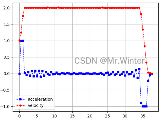
3.2 Python仿真
核心代码如下所示:
def process(self, path: List[Point3d]) –> List[Dict]:
velocity_profiles = []
path_segs, path_refs = PathPlanner.getPathSegments(path)
for i, path_seg in enumerate(path_segs):
s_ref = path_refs[i]
n = max(
len(path_refs[i]),
round(
self.r * (self.dx_max ** 2 + s_ref[–1] * self.ddx_max) \\
/ (self.dx_max * self.ddx_max * self.dt)
)
)
s_ref = np.linspace(0, s_ref[–1], n)
'''
min x^T P x + q^T x
s.t. l <= Ax <= u
'''
P = sparse.csc_matrix(self.calKernel(n))
q = self.calOffset(n, s_ref)
A = sparse.csc_matrix(self.calAffineConstraint(n))
l, u = self.calBoundary(n, s_ref)
solver = osqp.OSQP()
solver.setup(P, q, A, l, u, verbose=False)
res = solver.solve()
sol = res.x
velocity_profiles.append({
"time": [self.dt * i for i in range(n)],
"path": PathPlanner.pathInterpolation(path_seg, n),
"distance": sol[:n].tolist(),
"velocity": sol[n:2 * n].tolist(),
"acceleration": sol[2 * n:3 * n].tolist(),
})
return velocity_profiles
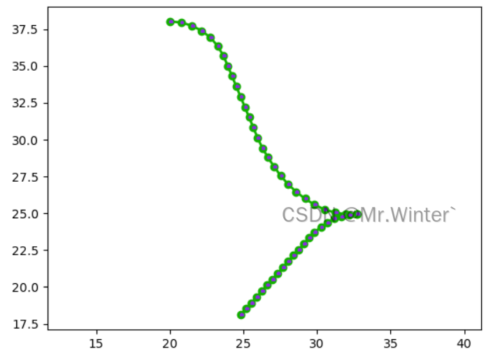
对于如下图所示的倒车路径
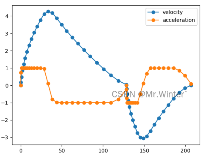
规划的速度和加速度曲线如下所示,中间速度为0处为换挡点
🔥 更多精彩专栏:
- 《ROS从入门到精通》
- 《Pytorch深度学习实战》
- 《机器学习强基计划》
- 《运动规划实战精讲》
- …
👇源码获取 · 技术交流 · 抱团学习 · 咨询分享 请联系👇


评论前必须登录!
注册