机器学习分类算法一——决策树

一、算法原理

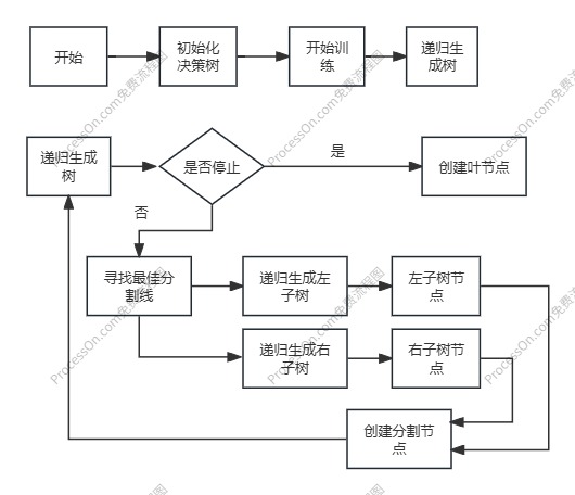
决策树算法通过将数据集划分为不同的子集来预测目标变量。它从根节点开始，根据某个特征对数据集进行划分，然后递归地生成更多的子节点，直到满足停止条件为止。决策树的每个内部节点表示一个特征属性上的判断条件，每个分支代表一个可能的属性值，每个叶节点表示一个分类结果。

二、参考代码

import numpy as np
import matplotlib.pyplot as plt

class TreeNode:
def __init__(self, feature_idx=None, threshold=None, left=None, right=None, class_dist=None):
self.feature_idx = feature_idx # 分割特征索引
self.threshold = threshold # 分割阈值
self.left = left # ≤ threshold 的子树
self.right = right # > threshold 的子树
self.class_dist = class_dist # 叶子节点的类别分布（用于预测）

class SimpleDecisionTree:
def __init__(self, max_depth=3):
self.max_depth = max_depth
self.tree = None
self.n_features = None

def fit(self, X, y):
y = np.asarray(y).astype(int) # 确保 y 是整数

self.n_features = X.shape[1]
self.tree = self._grow_tree(X, y, depth=0)

def _grow_tree(self, X, y, depth):
n_samples, n_features = X.shape
n_classes = len(np.unique(y))

# 停止条件：达到最大深度或所有样本属于同一类别
if depth >= self.max_depth or n_classes == 1:
class_dist = np.bincount(y, minlength=2)
return TreeNode(class_dist=class_dist)

# 寻找最佳分割
best_feature, best_threshold = self._best_split(X, y)

# 递归生长左右子树
left_idx = X[:, best_feature] <= best_threshold
right_idx = ~left_idx
left = self._grow_tree(X[left_idx], y[left_idx], depth + 1)
right = self._grow_tree(X[right_idx], y[right_idx], depth + 1)

return TreeNode(best_feature, best_threshold, left, right)

def _best_split(self, X, y):
best_gini = float('inf')
best_feature, best_threshold = None, None

for feature_idx in range(self.n_features):
thresholds = np.unique(X[:, feature_idx])
for threshold in thresholds:
gini = self._gini_impurity(X[:, feature_idx], y, threshold)
if gini < best_gini:
best_gini = gini
best_feature = feature_idx
best_threshold = threshold

return best_feature, best_threshold

def _gini_impurity(self, feature_col, y, threshold):
left_idx = feature_col <= threshold
right_idx = ~left_idx

if np.sum(left_idx) == 0 or np.sum(right_idx) == 0:
return float('inf')

left_dist = np.bincount(y[left_idx], minlength=2)
right_dist = np.bincount(y[right_idx], minlength=2)

left_prob = left_dist / np.sum(left_dist)
right_prob = right_dist / np.sum(right_dist)

gini_left = 1 – np.sum(left_prob ** 2)
gini_right = 1 – np.sum(right_prob ** 2)

total_gini = (np.sum(left_idx) * gini_left + np.sum(right_idx) * gini_right) / len(y)
return total_gini

def predict(self, X):
return np.array([self._predict_single(x, self.tree) for x in X])

def _predict_single(self, x, node):
if node.feature_idx is None: # 叶子节点
return np.argmax(node.class_dist)
if x[node.feature_idx] <= node.threshold:
return self._predict_single(x, node.left)
else:
return self._predict_single(x, node.right)

def visualize_tree(self, feature_names=None, class_names=None):
if feature_names is None:
feature_names = [f"Feature {i}" for i in range(self.n_features)]
if class_names is None:
class_names = ["no", "yes"]

fig, ax = plt.subplots(figsize=(10, 6))
ax.axis("off")

# 动态计算树的高度（递归深度）
def calc_depth(node):
if node is None:
return 0
left_depth = calc_depth(node.left)
right_depth = calc_depth(node.right)
return max(left_depth, right_depth) + 1

tree_depth = calc_depth(self.tree)

# 递归绘制节点（动态调整位置）
def _draw_node(node, x, y, x_offset, y_step, depth):
if node is None:
return

# 绘制当前节点
if node.feature_idx is not None: # 分割节点
ax.text(
x,
y,
f"{feature_names[node.feature_idx]} ≤ {node.threshold:.1f}",
ha="center",
va="center",
bbox=dict(facecolor="white", edgecolor="black", boxstyle="round"),
)
else: # 叶子节点
class_idx = np.argmax(node.class_dist)
class_label = class_names[class_idx]
n_samples = np.sum(node.class_dist)
prob = node.class_dist[class_idx] / n_samples
ax.text(
x,
y,
f"Predict: {class_label}\\n(n={n_samples}, p={prob:.2f})",
ha="center",
va="center",
bbox=dict(
facecolor="lightgreen" if class_idx == 1 else "lightcoral",
edgecolor="black",
boxstyle="round",
),
)

# 递归绘制子节点（动态调整位置）
if node.left or node.right:
_draw_node(node.left, x – x_offset, y – y_step, x_offset / 2, y_step, depth + 1)
_draw_node(node.right, x + x_offset, y – y_step, x_offset / 2, y_step, depth + 1)

# 绘制带箭头的连线
ax.annotate(
"",
xy=(x – x_offset, y – y_step + 0.1),
xytext=(x, y – 0.1),
arrowprops=dict(arrowstyle="->", color="blue"),
)
ax.annotate(
"",
xy=(x + x_offset, y – y_step + 0.1),
xytext=(x, y – 0.1),
arrowprops=dict(arrowstyle="->", color="red"),
)

# 初始位置和步长（缩小间距）
initial_x_offset = 0.5 / tree_depth # 根据树深度动态调整
y_step = 1 / tree_depth # 垂直间距
_draw_node(self.tree, x=0.5, y=0.9, x_offset=initial_x_offset, y_step=y_step, depth=0)

plt.tight_layout()
plt.show()

三、代码分析

1、决策树生成逻辑

在这里插入图片描述

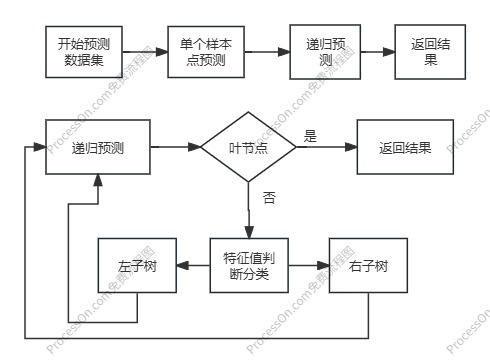
2、决策树预测逻辑

在这里插入图片描述

3、最佳分割线

def _best_split(self, X, y):
best_gini = float('inf')
best_feature, best_threshold = None, None

return best_feature, best_threshold

def _gini_impurity(self, feature_col, y, threshold):
left_idx = feature_col <= threshold
right_idx = ~left_idx

if np.sum(left_idx) == 0 or np.sum(right_idx) == 0:
return float('inf')

left_dist = np.bincount(y[left_idx], minlength=2)
right_dist = np.bincount(y[right_idx], minlength=2)

left_prob = left_dist / np.sum(left_dist)
right_prob = right_dist / np.sum(right_dist)

gini_left = 1 – np.sum(left_prob ** 2)
gini_right = 1 – np.sum(right_prob ** 2)

total_gini = (np.sum(left_idx) * gini_left + np.sum(right_idx) * gini_right) / len(y)
return total_gini

（1）Gini不纯度

定义：Gini 不纯度衡量的是一个数据集中随机选取两个样本，其类别不一致的概率。公式：

−

∑

Gini =1-\\sum_{k=1}^{K}p_k^2

$G ini = 1 - \sum_{k = 1}^{K} p_{k}^{2}$ 其中，其中：K是类别总数（如二分类问题中 K=2）。

p_k

$p_{k}$ 是第 k类样本在数据集中的比例。计算步骤：

1）选择一个分割特征和阈值

如age ≤ 40

2）划分数据：

左子集：满足条件的数据（age ≤ 40）。右子集：不满足条件的数据（age > 40）。

3）计算左右子集的 Gini 不纯度：

对左子集和右子集分别计算 Gini 不纯度。

4）计算加权平均 Gini 不纯度：

∗

Totel \\_ Gini=\\frac{n_{left}}{n_{totel}}*Gini_{left}+\\frac{n_{right}}{n_{totel}}*Gini_{right}

$T o t e l_G ini = \frac{n _{l e f t}}{n _{t o t e l}} * G in i_{l e f t} + \frac{n _{r i g h t}}{n _{t o t e l}} * G in i_{r i g h t}$ 其中,

、

n_{right}、n_{left}、n_{totel}

$n_{r i g h t} 、 n_{l e f t} 、 n_{t o t e l}$ 分别为左子集、右子集和总集的样本个数。

参考文献

1、【总结】机器学习中的15种分类算法

机器学习分类算法一——决策树

一、算法原理

二、参考代码