 网硕互联帮助中心
代码来自https://github.com/idies/pyJHTDB/blob/master/examples/channel.ipynb
%matplotlib inline
import numpy as np
import math
import random
import pyJHTDB
import matplotlib.pyplot as plt
import time as tt
N = 3
T = pyJHTDB.dbinfo.channel5200['time'][-1]
time = np.random.random()*T
spatialInterp = 6 # 6 拉格朗日点
temporalInterp = 0 # 无时间插值
FD4Lag4 = 44 # 4 point Lagrange interp for derivatives
# mhdc has starttime .364 and endtime .376
startTime = time
endTime = startTime + 0.012
lag_dt = 0.0004
# Select points in the database to query
lpoints = []
for i in range(0,N):
lpoints.append([random.uniform(0, 8*3.14),random.uniform(-1, 1),random.uniform(0, 3*3.14)])
# 2D array with single precision values
points = np.array(lpoints,dtype='float32')
# load shared library
lTDB = pyJHTDB.libJHTDB()
#initialize webservices
lTDB.initialize()
#Add token
auth_token = "edu.jhu.pha.turbulence.testing-201311" #Replace with your own token here
lTDB.add_token(auth_token)
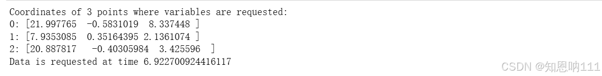
print('Coordinates of {0} points where variables are requested:'.format(N))
for p in range(N):
print('{0}: {1}'.format(p, points[p]))
print('Data is requested at time {0}'.format(time))
下面是逐行分析
- %matplotlib inline:在 Jupyter Notebook 中使 matplotlib 的图表内嵌显示。
- numpy、math、random:用于数学运算和随机数生成。
- pyJHTDB:用于访问 Johns Hopkins 湍流数据库 (JHTDB) 的 Python 包。
- matplotlib.pyplot:用于绘图。
- time:用于计时。
N = 3
T = pyJHTDB.dbinfo.channel5200['time'][-1]
time = np.random.random()*T
说明:
- N = 3:定义了要查询的点的数量。
- T = pyJHTDB.dbinfo.channel5200['time'][-1]:获取 channel5200 数据集中时间序列的最后一个时间点,表示整个时间范围。
- time = np.random.random() * T:生成一个随机的时间 time,范围从 0 到 T。
spatialInterp = 6 # 6 拉格朗日点
temporalInterp = 0 # 无时间插值
FD4Lag4 = 44 # 4 point Lagrange interp for derivatives
- spatialInterp = 6:设置空间插值类型为 6 点拉格朗日插值。
- temporalInterp = 0:时间插值设为无插值。
- FD4Lag4 = 44:用于计算导数的 4 点拉格朗日插值。
startTime = time
endTime = startTime + 0.012
lag_dt = 0.0004
说明:
- startTime = time:设置查询的开始时间。
- endTime = startTime + 0.012:设置查询的结束时间,时间范围为 0.012 单位。
- lag_dt = 0.0004:设置时间步长为 0.0004。
lpoints = []
for i in range(0, N):
lpoints.append([random.uniform(0, 8*3.14), random.uniform(-1, 1), random.uniform(0, 3*3.14)])
说明:
- 初始化 lpoints 为一个空列表。
- 使用循环生成 N 个随机的坐标点,每个点是一个 [x, y, z] 的三维位置:
- x 范围在 0 到 8π。
- y 范围在 -1 到 1。
- z 范围在 0 到 3π。
points = np.array(lpoints, dtype='float32')
lTDB = pyJHTDB.libJHTDB()
lTDB.initialize()
说明:
- 将 lpoints 转换为单精度浮点型的 NumPy 数组 points,用于之后的查询。
- lTDB = pyJHTDB.libJHTDB():创建 libJHTDB 类的实例 lTDB,用于访问 JHTDB。
- lTDB.initialize():初始化 JHTDB 服务,准备进行数据查询。
auth_token = "edu.jhu.pha.turbulence.testing-201311" #Replace with your own token here
lTDB.add_token(auth_token)
print('Coordinates of {0} points where variables are requested:'.format(N))
for p in range(N):
print('{0}: {1}'.format(p, points[p]))
print('Data is requested at time {0}'.format(time))
说明:
- auth_token:设置授权令牌,用于访问 JHTDB 服务。
- 如何将auth_token更换为自己的???
- lTDB.add_token(auth_token):将授权令牌添加到 lTDB 实例,确保能够进行查询
- 打印出 N 个点的坐标,显示每个点的位置。
- 打印查询数据的随机时间 time。
这段代码的作用是:
- 导入必要的库和模块。
- 生成 N 个随机的三维点,用于查询湍流数据库中的物理变量。
- 设置插值和查询参数。
- 初始化和授权 JHTDB 服务。
- 打印出查询的坐标和时间,以便用户确认。
这段代码用于从 JHTDB 获取在特定时间和空间位置上的湍流数据,接下来可以调用相关方法来获取数据并进行分析。
print('Requesting pressure at {0} points…'.format(N))
result = lTDB.getData(time, points,data_set = 'channel',
sinterp = spatialInterp, tinterp = temporalInterp,
getFunction = 'getPressure')
for p in range(N):
print('{0}: {1}'.format(p, result[p]))
说明:
- result 变量接收从 JHTDB 查询得到的数据。
- lTDB.getData() 是 libJHTDB 类中的方法,用于从数据库中获取物理量数据。以下是各参数的含义:
- time:请求数据的时间。
- points:一个包含查询空间位置的数组,即前面生成的 N 个随机点。
- data_set='channel':指定使用的湍流数据集,这里是 channel 数据集。
- 想获取别的数据集数据时如何知道别的数据集名称???
- sinterp=spatialInterp:指定空间插值方法,这里使用的是 6 点拉格朗日插值。
- tinterp=temporalInterp:指定时间插值方法,这里不使用时间插值。
- 插值法的作用是什么?为什么要插值???
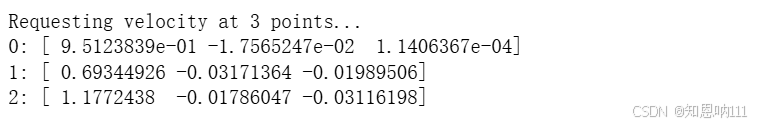
- getFunction='getVelocity':指定要获取的数据是速度信息。
- 遍历 result 数组并打印每个点的结果。
- '{0}: {1}'.format(p, result[p]) 格式化输出,显示点的索引和对应的速度值。
总结
这段代码的作用是:
- 从 JHTDB 请求特定时间和空间位置的速度数据。
- 使用 getData() 方法进行查询。
- 输出每个查询点的速度结果,方便用户查看和验证。
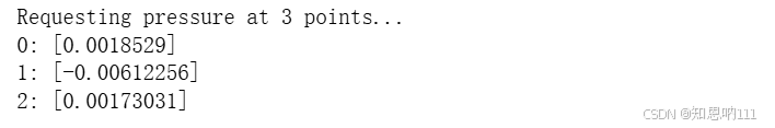
print('Requesting pressure at {0} points…'.format(N))
result = lTDB.getData(time, points,data_set = 'channel',
sinterp = spatialInterp, tinterp = temporalInterp,
getFunction = 'getPressure')
for p in range(N):
print('{0}: {1}'.format(p, result[p]))
同理,这段代码获取的压力值
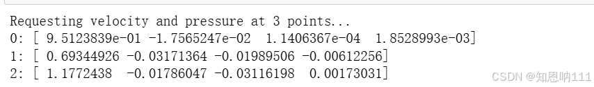
print('Requesting velocity and pressure at {0} points…'.format(N))
result = lTDB.getData(time, points,data_set = 'channel',
sinterp = spatialInterp, tinterp = temporalInterp,
getFunction = 'getVelocityAndPressure')
for p in range(N):
print('{0}: {1}'.format(p, result[p]))
这段代码获取的速度和压力值
print('Requesting velocity gradient at {0} points…'.format(N))
result = lTDB.getData(time, points,
sinterp = FD4Lag4, tinterp = temporalInterp,data_set ='channel',
getFunction = 'getVelocityGradient')
for p in range(N):
print('{0}: '.format(p) +
'duxdx = {0:+e}, duxdy = {1:+e}, duxdz = {2:+e}\\n '.format(result[p][0], result[p][1], result[p][2]) +
'duydx = {0:+e}, duydy = {1:+e}, duydz = {2:+e}\\n '.format(result[p][3], result[p][4], result[p][5]) +
'duzdx = {0:+e}, duzdy = {1:+e}, duzdz = {2:+e}'.format(result[p][6], result[p][7], result[p][8]))
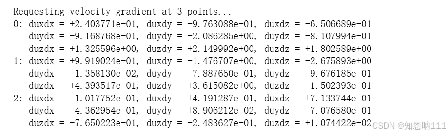
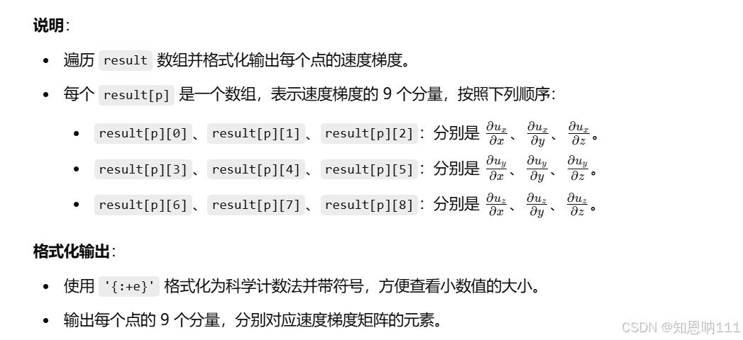
说明:
- 调用 lTDB.getData() 函数来获取速度梯度数据。
- getFunction='getVelocityGradient':表示要获取速度梯度信息。
- 遍历 result 数组,并格式化输出每个点的速度梯度。
- result[p] 包含当前点的速度梯度,排列方式为 [duxdx, duxdy, duxdz, duydx, duydy, duydz, duzdx, duzdy, duzdz],分别表示速度分量 u、v、w 在 x、y、z方向上的偏导数。
print('Requesting velocity hessian at {0} points…'.format(N))
result = lTDB.getData(time, points,data_set = 'channel',sinterp = FD4Lag4, tinterp = temporalInterp,
getFunction = 'getVelocityHessian')
for p in range(N):
print('{0}: '.format(p) +
'd2uxdxdx = {0:+e}, d2uxdxdy = {1:+e}, d2uxdxdz = {2:+e}\\n '.format(result[p][ 0], result[p][ 1], result[p][ 2])
+ 'd2uxdydy = {0:+e}, d2uxdydz = {1:+e}, d2uxdzdz = {2:+e}\\n '.format(result[p][ 3], result[p][ 4], result[p][ 5])
+ 'd2uydxdx = {0:+e}, d2uydxdy = {1:+e}, d2uydxdz = {2:+e}\\n '.format(result[p][ 6], result[p][ 7], result[p][ 8])
+ 'd2uydydy = {0:+e}, d2uydydz = {1:+e}, d2uydzdz = {2:+e}\\n '.format(result[p][ 9], result[p][10], result[p][11])
+ 'd2uzdxdx = {0:+e}, d2uzdxdy = {1:+e}, d2uzdxdz = {2:+e}\\n '.format(result[p][12], result[p][13], result[p][14])
+ 'd2uzdydy = {0:+e}, d2uzdydz = {1:+e}, d2uzdzdz = {2:+e}'.format(result[p][15], result[p][16], result[p][17]))
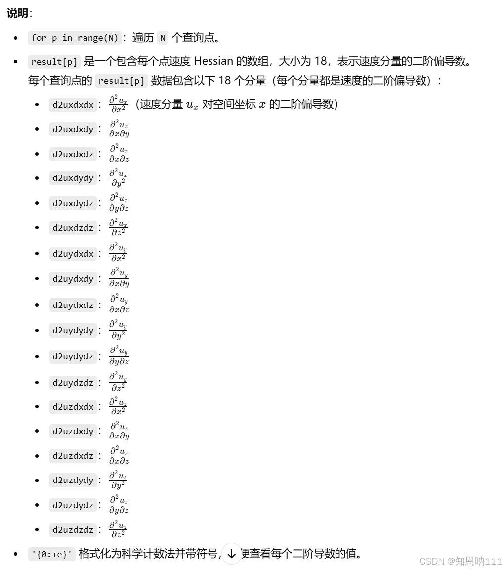
获取速度的二阶导数
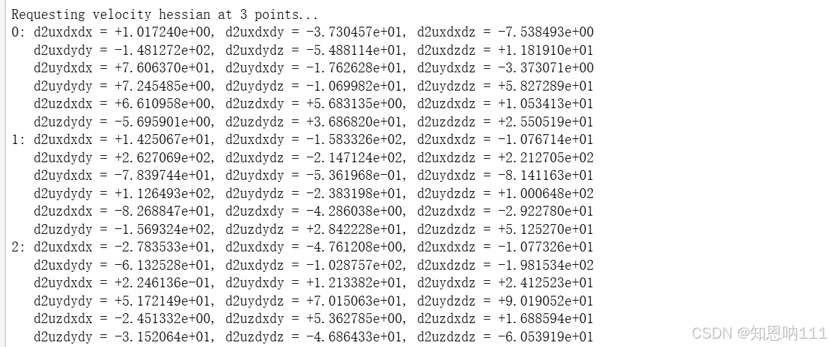
说明:
- result 变量接收从 JHTDB 查询得到的速度 Hessian 数据。
- lTDB.getData() 方法用于从数据库中获取数据,参数含义如下:
- time:请求数据的时间。
- points:一个包含查询空间位置的数组,即你之前生成的随机点。
- data_set='channel':指定数据集,这里使用的是 channel 数据集。
- sinterp=FD4Lag4:使用 4 点拉格朗日插值(FD4Lag4)计算导数,用于计算 Hessian。
- tinterp=temporalInterp:指定时间插值方法,这里不使用时间插值(设为 0)。
- getFunction='getVelocityHessian':指定要获取的数据是速度 Hessian。
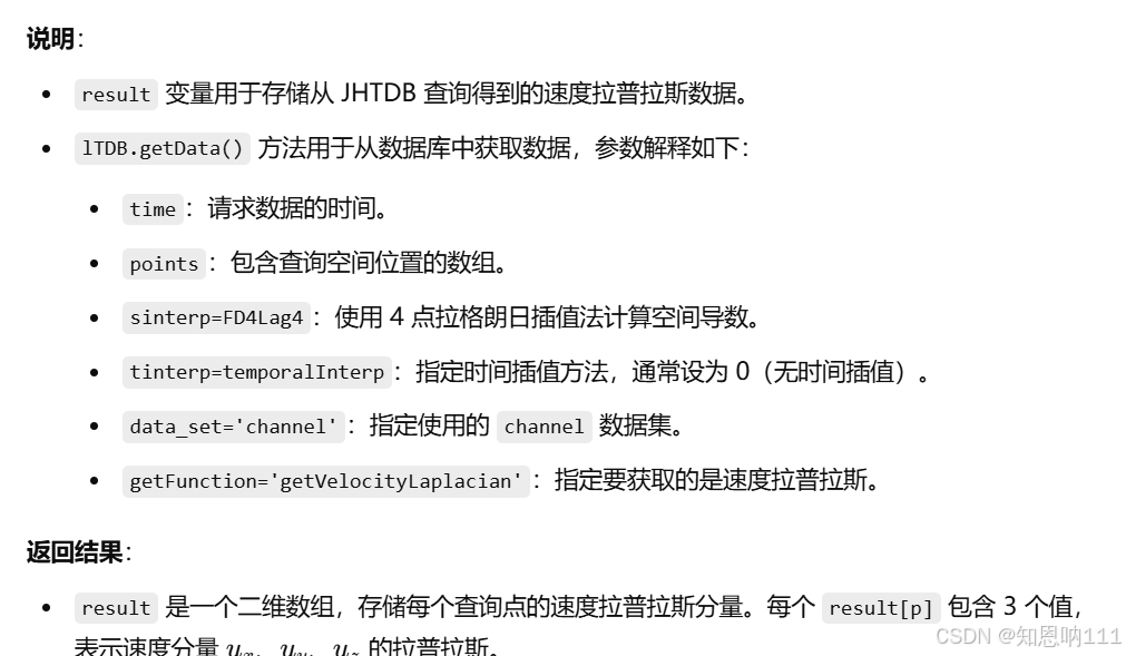
print('Requesting velocity laplacian at {0} points…'.format(N))
result = lTDB.getData(time, points,
sinterp = FD4Lag4, tinterp = temporalInterp, data_set = 'channel',
getFunction = 'getVelocityLaplacian')
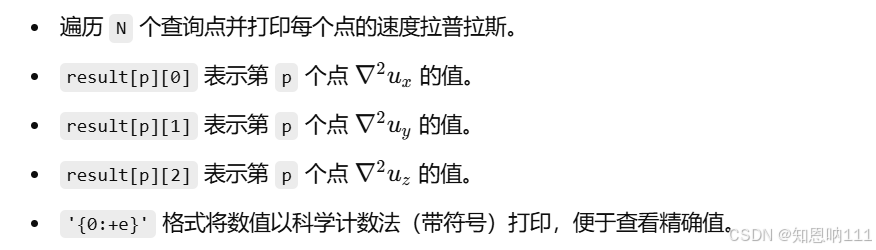
for p in range(N):
print('{0}: '.format(p) +
'grad2ux = {0:+e}, grad2uy = {1:+e}, grad2uz = {2:+e}, '.format(result[p][0], result[p][1], result[p][2]))
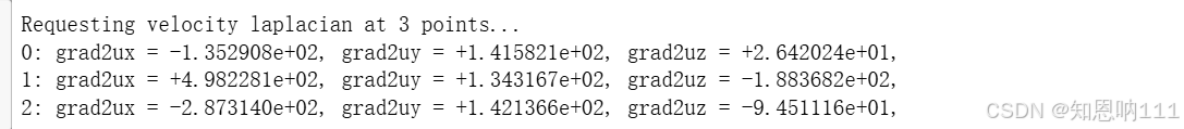
标输出结果解释
print('Requesting pressure hessian at {0} points…'.format(N))
result = lTDB.getData(time, points,
sinterp = FD4Lag4, tinterp = temporalInterp, data_set = 'channel',
getFunction = 'getPressureHessian')
for p in range(N):
print('{0}: '.format(p) +
'd2pdxdx = {0:+e}, d2pdxdy = {1:+e}, d2pdxdz = {2:+e}\\n '.format(result[p][0], result[p][1], result[p][2])
+ 'd2pdydy = {0:+e}, d2pdydz = {1:+e}, d2pdzdz = {2:+e}'.format(result[p][3], result[p][4], result[p][5]))
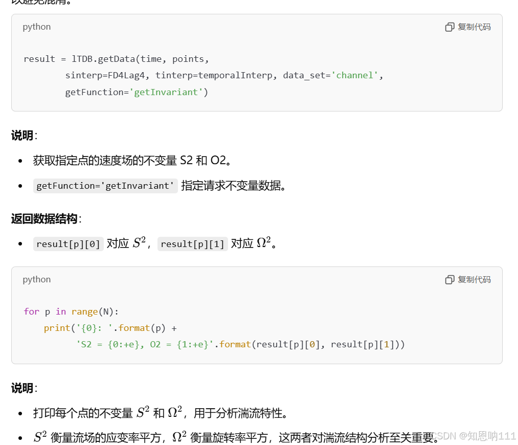
print('Requesting pressure hessian at {0} points…'.format(N))
result = lTDB.getData(time, points,
sinterp = FD4Lag4, tinterp = temporalInterp, data_set = 'channel',
getFunction = 'getInvariant')
for p in range(N):
print('{0}: '.format(p) +
'S2 = {0:+e}, O2 = {1:+e}'.format(result[p][0], result[p][1]))
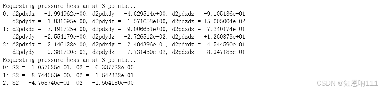
说明:
- 从数据库中获取指定时间和位置的压力 Hessian。
- getFunction='getPressureHessian' 指定请求的是压力的 Hessian 数据。
返回数据结构:
- result[p] 包含每个查询点的 6 个分量,对应 Hessian 矩阵中不重复的上三角部分。
- 打印每个点的压力 Hessian 分量。
- result[p][0] 表示 ∂2p∂x2\\frac{\\partial^2 p}{\\partial x^2}∂x2∂2p,依次类推。
- 使用科学计数法格式化输出,使结果更清晰。

result = lTDB.getThreshold(
data_set = 'channel',
field = 'vorticity',
time = 0,
threshold = 65,
x_start = 1, y_start = 1, z_start = 1,
x_end = 4, y_end = 4, z_end = 4,
sinterp = 40,
tinterp = 0)
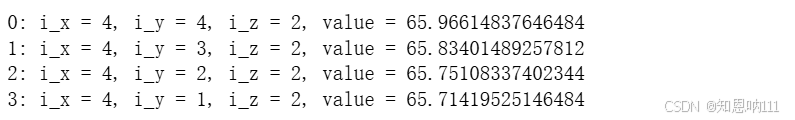
for p in range(result.shape[0]):
print('{0}: '.format(p)
+ 'i_x = {0}, i_y = {1}, i_z = {2}, value = {3} '.format(result[p][0], result[p][1], result[p][2],result[p][3]))
逐句分析
result = lTDB.getThreshold(…):
- 使用 getThreshold 方法,从指定的 data_set(此处是 'channel')中获取满足特定阈值条件的涡量场('vorticity')数据点。
- 参数 time = 0 指定在时间 t=0 时刻获取数据。
- 参数 threshold = 65 表示提取涡量值大于或等于 65 的点。
- x_start, y_start, z_start 和 x_end, y_end, z_end 定义了要查询的立方体区域在网格中的起始和结束索引范围。
- sinterp = 40 表示用于空间插值的方法。
- tinterp = 0 表示没有时间插值。
for p in range(result.shape[0])::
- 遍历 result 数组的每个数据点。result 中的每个元素对应一个满足阈值条件的点。
print(…):
- 打印每个满足条件的点的索引和涡量值。
- i_x, i_y, i_z 表示该点在网格中的索引位置。
- value 表示该点的涡量值。
解释用途
- 寻找高涡量区域:此方法有助于在流场中定位具有强旋转运动(高涡量)的区域,这些区域通常与湍流结构相关联,如涡核或强旋涡。
- 研究湍流结构:提取和分析高涡量点可以帮助研究人员更好地理解湍流的特征,如旋涡生成和消散的机制。
-
举例说明
假设你在一个流动实验中想找到所有具有较高旋转速率的点,比如模拟中能量较集中的旋涡结构,这段代码会帮你在指定的立方体区域内找到涡量大于等于 65 的点,并返回这些点的网格位置和涡量值。
start = tt.time()
result = lTDB.getCutout(
data_set = 'channel',
field='u',
time_step=int(1),
start = np.array([1, 1, 1], dtype = int),
end = np.array([512, 512, 1], dtype = int),
step = np.array([1, 1, 1], dtype = int),
filter_width = 1)
#print(result)
end = tt.time()
print(end – start)
(这里使用 np.array([512, 512, 1],服务器会崩,不知道为什么,100都不行???问题已解决:由于token用的测试token(只能提取小切片),需要主动申请一个token)
这段代码的作用是从指定的湍流数据集中提取特定区域的速度场数据(field='u' 表示获取速度场的 u 分量)。下面是详细的逐句分析和解释:
逐句分析
start = tt.time():
- 记录当前时间戳,以测量获取数据所需的时间。
result = lTDB.getCutout(…):
- 使用 getCutout 方法从 channel 数据集中提取指定的切片数据。
- 参数说明:
- data_set = 'channel':指定从通道湍流数据集中获取数据。
- field='u':选择提取的场为速度的 uuu 分量(通常代表流动的 x 方向分量)。
- time_step=int(1):选择时间步为 1。
- start = np.array([1, 1, 1], dtype = int):起始位置,表示从网格中的第一个点(x=1, y=1, z=1)开始。
- end = np.array([512, 512, 1], dtype = int):结束位置,表示在 x 和 y 方向扩展到 512,z 方向只取一个平面。
- step = np.array([1, 1, 1], dtype = int):步长为 1,意味着在每个方向上提取连续数据点。
- filter_width = 1:表示用于数据提取的过滤器宽度。
#print(result):
- 这行被注释掉了,通常用于查看结果数组的内容。可以取消注释以调试或查看数据提取结果。
end = tt.time():
- 记录数据提取完成后的时间戳。
print(end – start):
- 打印提取数据所花费的总时间,以秒为单位。这有助于评估从数据库提取数据的效率。
解释用途
这段代码旨在从湍流数据库中提取一个平面切片的数据(在 z=1 位置上、整个 x 和 y 平面的 uuu 分量)。提取这样的切片数据可以用于可视化流场的某一层,或者进一步的流动分析,例如涡结构检测或速度分布研究。
示例用途
例如,你想观察湍流通道中某一个特定平面上的速度分布,或者进行二维的流动分析(如流线图或速度图),这段代码会帮助你快速提取所需的数据切片进行分析。
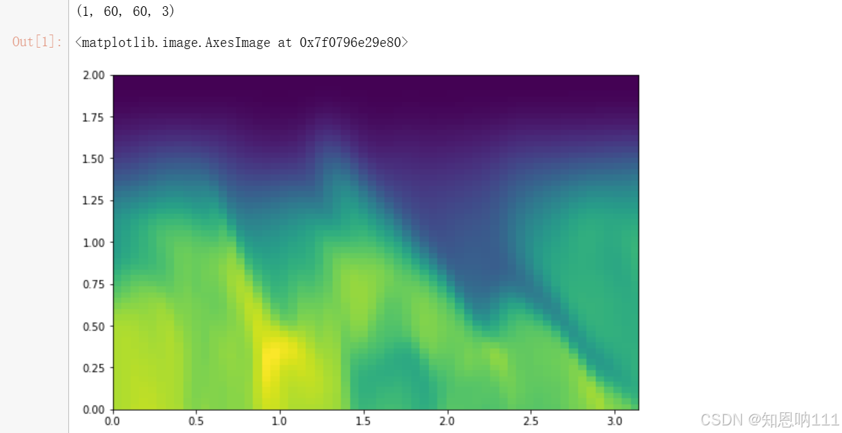
print(result.shape)
fig = plt.figure(figsize = (20, 40))
a = fig.add_subplot(121)
#a.set_axis_off()
a.imshow(result[0,:,:,0],
extent = [0, 3.14, 0, 2],
interpolation = 'none')
x, t = lTDB.getPosition(
starttime = 0.1,
endtime = 0.2,
dt = 0.01,
data_set = 'channel',
point_coords = points[0:1,:],
steps_to_keep = 10)
print(x)
这段代码的作用是可视化从湍流数据库中提取的速度场数据。下面是逐句分析和解释:
逐句分析
print(result.shape):
- 打印提取结果 result 的形状,用于确认数据的维度和大小。输出的形状会告诉你数据在 x、y、z方向上的采样点数及其结构。
fig = plt.figure(figsize = (20, 40)):
- 创建一个 Matplotlib 图形对象 fig,设置图形的大小为 20 × 40 英寸。较大的尺寸通常用于高分辨率的显示或打印。
a = fig.add_subplot(121):
- 添加一个子图 a 到图形 fig 中。121 表示图像布局为 1 行 2 列,并选择第 1 个子图。
a.imshow(result[0,:,:,0], extent = [0, 3.14, 0, 2], interpolation = 'none'):
- 使用 imshow 方法在子图 a 上显示数据切片。
- result[0,:,:,0]:提取 result 中 z=1 处的 uuu 分量(整个 x 和 y 平面上的数据)。
- extent = [0, 3.14, 0, 2]:指定显示范围,将 x 轴范围映射到 [0, 3.14],y 轴范围映射到 [0, 2]。这些值通常根据实际物理空间进行映射。
- interpolation = 'none':不进行插值,直接显示原始数据点。
x, t = lTDB.getPosition(
starttime = 0.1,
endtime = 0.2,
dt = 0.01,
data_set = 'channel',
point_coords = points[0:1,:],
steps_to_keep = 10)
print(x)
这段代码使用了 lTDB.getPosition() 方法来追踪流体中的点随时间的移动,具体解释如下:
逐句分析
x, t = lTDB.getPosition(…):
- 调用 getPosition 方法来获取指定点在流场中随着时间演化的位置轨迹。
- 返回值 x 是一个包含点在各个时间步的空间坐标的数组,t 是对应的时间步数组。
starttime = 0.1, endtime = 0.2:
- starttime 和 endtime 指定了位置追踪的时间范围,从 0.1 到 0.2(时间的单位取决于数据集的定义,如秒或无量纲时间)。
dt = 0.01:
- 设置每个时间步长为 0.01,这表示在 starttime 和 endtime 之间,每隔 0.01 个时间单位计算一次点的位置。
data_set = 'channel':
- 表示使用的流场数据集是 'channel'。
point_coords = points[0:1,:]:
- 选择 points 数组中的第一个点(points[0])作为起始位置进行追踪。[0:1, :] 表示只取第一个点的全部坐标(x, y, z)。
steps_to_keep = 10:
- 指定保存每隔多少个时间步的数据。例如,这个值为 10 表示程序会在 10 个计算步长中取 1 个位置来保存。
print(x):
- 打印 x,输出每个时间步中点的位置坐标。
代码用途
这段代码用于研究单个流体点在指定时间区间内的运动轨迹。输出的 x 是一个包含各个时间步位置坐标的数组,帮助研究人员了解在流场中点的移动情况。
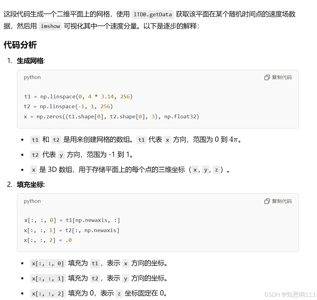
t1 = np.linspace(0, 4*3.14, 256)
t2 = np.linspace(-1, 1, 256)
x = np.zeros((t1.shape[0], t2.shape[0], 3), np.float32)
x[:, :, 0] = t1[np.newaxis, :]
x[:, :, 1] = t2[:, np.newaxis]
x[:, :, 2] = .0
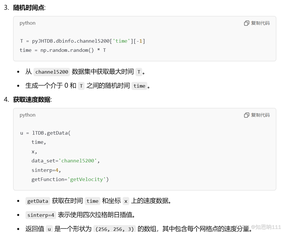
T = pyJHTDB.dbinfo.channel5200['time'][-1]
time = np.random.random()*T
u = lTDB.getData(
time,
x,
data_set = 'channel5200',
sinterp = 4,
getFunction='getVelocity')
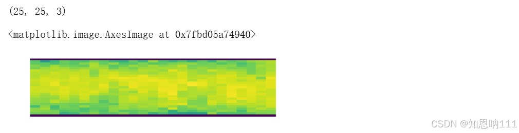
print(u.shape)
fig = plt.figure(figsize = (t1[-1] – t1[0], t2[-1] – t2[0]))
a = fig.add_subplot(121)
a.set_axis_off()
a.imshow(u[:,:,0],
extent = [t1[0], t1[-1] – t1[0], t2[0], t2[-1] – t2[0]],
interpolation = 'none')
 最后
最后
lTDB.finalize()
##是用于释放资源、关闭与数据服务器的连接或清理与 lTDB(如 PyJHTDB 类库)相关的会话的命令。


评论前必须登录!
注册