 网硕互联帮助中心
超详细指南:MATLAB 频域操控与信号恢复 —— 从零填充信号到削波基波提取
Ultra-Detailed Guide: Frequency-Domain Manipulation and Signal Recovery in MATLAB — From Zero-Padded Signals to Fundamental Extraction from Clipped Waveforms
🌐 English Version (Ultra-Detailed)
📌 Article Abstract (Directly Searchable)
This advanced guide focuses on inverse DFT operations — manipulating spectra to recover or transform time-domain signals. It addresses three classic tasks:
🛠️ Zero: Mathematical Prerequisites
- Conjugate Symmetry: For real signals, ( X[k] = X^*[N-k] ). Both positive and negative frequency bins must be preserved together.
- DFT Amplitude Scaling: For a pure sine of amplitude ( A ) and length ( N ), the positive-frequency FFT magnitude is ( A \\cdot N / 2 ). Zero-padding to length ( N_2 ) scales this value to ( A \\cdot N_2 / 2 ).
📝 Part 1: The reshape Magic & Sampling Analogy (Q1)
Task: Run the given code, observe the waveform, and explain its FFT.
Code dissection:
- z is a 2Hz cosine sampled at 128Hz (128 points).
- x = zeros(10,128); x(1,:)=z; creates a matrix with only the first row filled.
- reshape(x,1,1280) reads column by column. It outputs: [z(1), 0,0…0 (9 zeros), z(2), 0,0…0, …].
- Result: A 1-second burst of 2Hz cosine followed by 9 seconds of silence.
Analogy: This resembles pulse sampling or gated sampling in analog systems — the signal is visible only during a short duty cycle.
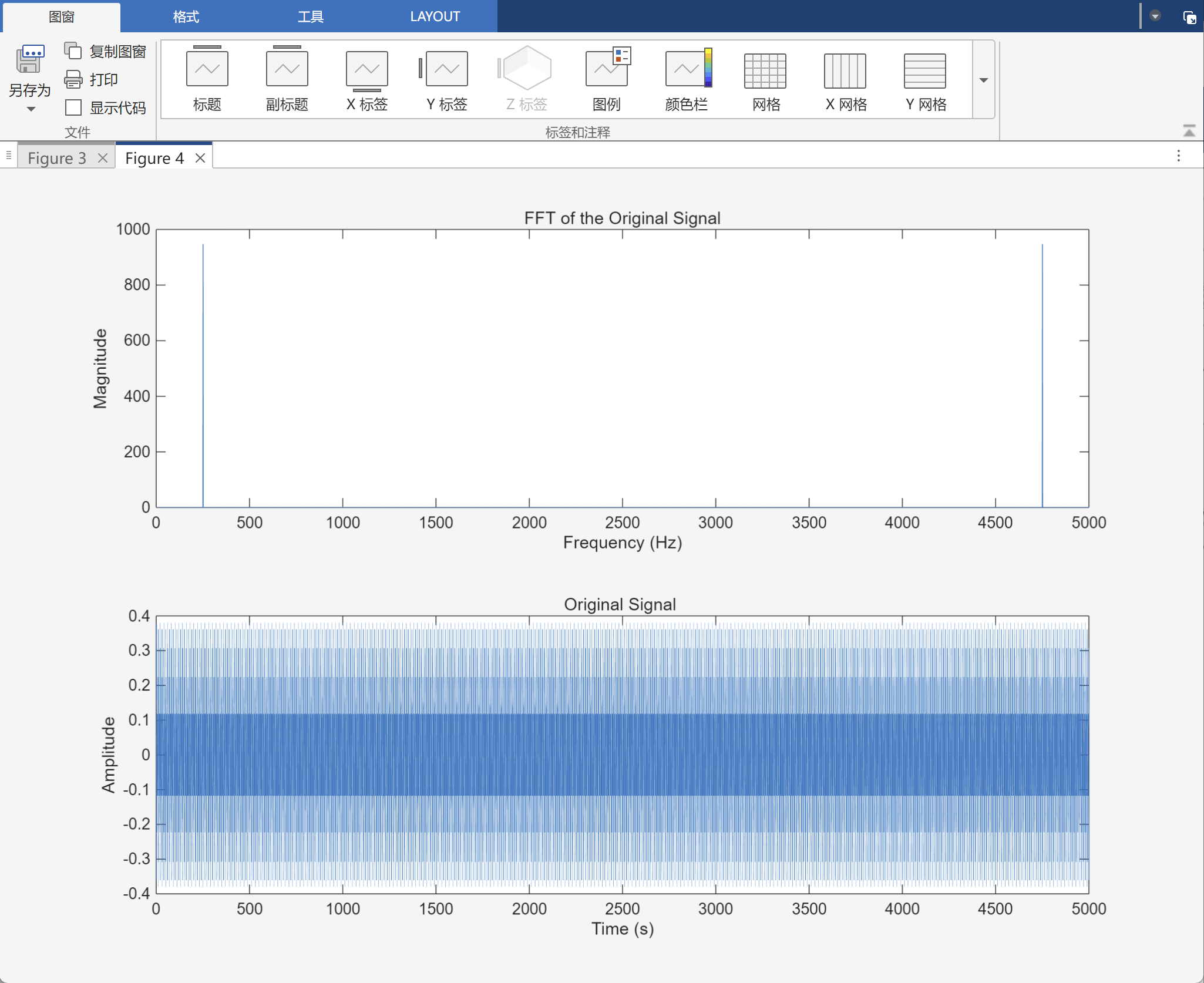
FFT Analysis: The spectrum shows a sinc-shaped main lobe centered at 2Hz, with interpolated side lobes due to zero-padding (10× higher frequency resolution).
📊 Part 2: Extracting a Continuous Sine (No Zero Insertion) — Q2
Task: Manipulate the FFT to recover a sine wave that is continuous over the whole time axis (no zeros), and explain its amplitude.
Correct Approach:
- Locate the exact positive and negative frequency bins for 2Hz in the 1280-point FFT.
- Zero-frequency indexing: 2Hz corresponds to normalized index ( 2/128 ). In 1280-point FFT, ( k = (2/128) \\times 1280 = 20 ) (0‑based), so MATLAB index = 21. Negative conjugate index = ( 1280 – 20 + 2 = 1262 ).
Correct Code:
X = fft(x);
X_clean = zeros(1,1280);
X_clean(21) = X(21);
X_clean(1262) = X(1262);
y = real(ifft(X_clean));
Amplitude Derivation (Crucial):
- Original 128-point FFT magnitude at 2Hz = ( 1 \\times 128 / 2 = 64 ).
- After zero-padding to 1280, the magnitude scales to ( 64 \\times (1280/128) = 640 ).
- IFFT with one conjugate pair yields amplitude = ( 2 \\times 640 / 1280 = 1.0 ).
- Conclusion: The recovered continuous sine has an amplitude of exactly 1.0, matching the original.
🎯 Part 3: Fundamental Extraction from Clipped Signal — Q3 (Real Recovery)
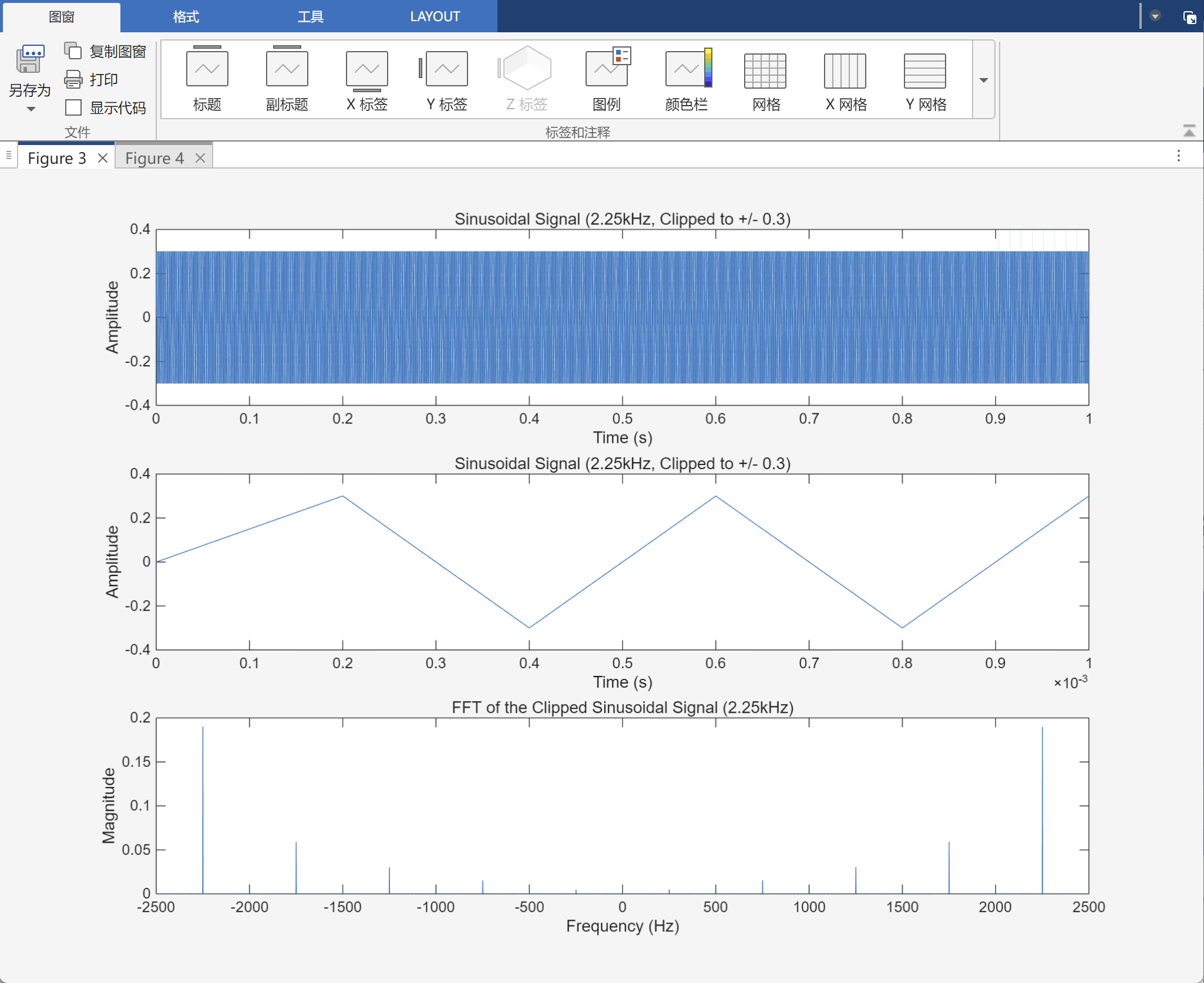
Task: From the 2.25kHz clipped signal (fs=5kHz, clipped to ±0.3), extract a clean sinusoid at the original frequency.
Feasibility: The clipped spectrum contains the fundamental (2.25kHz) and aliased harmonics (1.75k, 1.25k, etc.). They occupy distinct bins (resolution = 1Hz). We keep only the fundamental bin and discard all others.
Correct Code:
X = fft(signal); N = length(X); % N=5000
k_fund = round(2250 * 5000 / 5000) + 1; % = 2251
k_neg = N – k_fund + 2; % = 2751
X_clean = zeros(1,N);
X_clean(k_fund) = X(k_fund);
X_clean(k_neg) = X(k_neg);
recovered = real(ifft(X_clean));
Result Analysis:
- Waveform: Perfectly smooth sine at 2.25kHz.
- Amplitude: Approximately 0.7 (not 1.0). Why? Because clipping transferred part of the fundamental energy to harmonics. We extracted only the remaining fundamental component. To restore the original 1.0 amplitude, one would need prior knowledge of the clipping level and use nonlinear compensation (e.g., iterative algorithms), which is beyond linear frequency-domain bin selection.
🔍 Part 4: Dissecting Common Coding Mistakes (from your .m files)
Mistake 1: Zeroing a Wide Frequency Band (lab1bb.m Plan2)
clipping_range_indices = round([1000,3000]/freq_res)+1;
X(clipping_range_indices(1):clipping_range_indices(2)) = …
abs(X(clipping_range_indices(1):clipping_range_indices(2)));
Why wrong: This attempts a band-stop/band-modify filter, which corrupts phase and affects the fundamental itself (2250Hz lies inside 1000~3000Hz).
Mistake 2: Using Clipping Ratio to Define Cutoff (lab1b.m)
cut_ratio = 0.3 / 1;
N_cut = round(N/2) * cut_ratio;
X_cut(N_cut+1:end) = 0;
Why wrong: The clipping ratio determines time-domain peak truncation, not the frequency positions of harmonics. Aliased frequencies (1.75k, 1.25k) are determined by ( f_s ) and ( f ), not by the clipping threshold. This operation is essentially low-pass filtering, which cannot isolate the fundamental from in-band aliases.
Mistake 3: Operating on abs after fftshift (lab1bb2.m)
y2 = fftshift(abs(fft(signal)));
y2((5001–1)*0.1:(5001–1)*0.9) = 0;
Why wrong: abs destroys phase information. Zeroing a central band acts as a strange notch filter and cannot extract a single tone.
The Golden Rule: To extract a specific frequency, operate on a single complex bin (and its conjugate), not on a range of bins. This is equivalent to an ideal narrow-band filter with bandwidth ( \\Delta f ).
💎 Summary and Engineering Insights
| Recover continuous sine from zero-padded burst | Keep only the conjugate bins of the tone | Equal to original (1.0) | IFFT length must match FFT length |
| Recover fundamental from clipped signal | Keep only the fundamental conjugate bins | Equal to post-clipping fundamental amplitude (<1.0) | Cannot restore lost harmonic energy |
| General aliased component separation | Possible only if target and alias are in different bins | Depends on the actual component energy | If they share the same bin, separation is mathematically impossible |
Engineering Takeaway: Frequency-domain bin selection is a powerful tool for extracting known periodic components from distorted signals, widely used in power quality monitoring (fundamental extraction), ECG signal processing, and narrowband interference suppression. However, it fails when the sampling rate is too low to resolve the target and interfering frequencies into distinct bins.
📌 文章简介(可直接检索到题目)
本文是“信号采样与频谱分析”系列的进阶篇,聚焦于 离散傅里叶变换(DFT)的逆操作,即如何通过操控频谱来“改造”或“恢复”时域信号。内容严格对应以下三道经典任务:
🔬 零、预备知识与核心数学原理
在开始操作之前,必须深刻理解以下两条 DFT 性质:
- 共轭对称性:对于实信号,其 DFT 频谱满足 ( X[k] = X^*[N – k] )(其中 ( N ) 为 DFT 长度)。因此,保留一个正频率分量,必须同时保留其对应的负频率共轭分量,否则 IFFT 后会产生复数信号(虚部不为零)。
- DFT 幅度与正弦波幅度的关系:对于一个长度为 ( N )、幅度为 ( A ) 的纯正弦波 ( A \\cos(2\\pi f t) ),其单边未归一化 FFT 在正频率处的幅度为 ( A \\cdot N / 2 )。若将频谱长度从 ( N_1 ) 补零延长到 ( N_2 ),则该频点的幅度值会按比例变为 ( A \\cdot N_2 / 2 )(因为 FFT 算法默认不做能量归一化)。
📝 第一部分:reshape 的魔术与“采样”类比(对应 Q1)
任务描述
运行以下 MATLAB 代码,观察 Figure 1 中的信号“看起来像什么”——换句话说,它在哪些方面类似于模拟域中的采样信号?放大观察,并对 x 进行 FFT,解释你看到的现象。
x = zeros(10, 128);
t1 = 0:1/128:1–1/128;
z = cos(2 * pi * 2 * t1); % 2Hz 余弦,128 个采样点(采样率 128Hz)
x(1, :) = z; % 第一行存入余弦波
x = reshape(x, 1, 1280); % 将 10×128 矩阵重塑为 1×1280 的行向量
figure(1); plot(x);
代码逐步拆解与物理意义
生成基础信号 z:
- 采样率 ( f_{s1} = 128 \\text{ Hz} ),时长 1 秒,共 128 个点。
- 信号频率为 2 Hz,每个周期包含 ( 128 / 2 = 64 ) 个采样点,波形非常光滑。
构造矩阵 x:
- zeros(10, 128) 生成了一个 10 行、128 列的全零矩阵。
- 将 z 赋值给第一行(第 2~10 行保持全零)。
reshape 操作(关键):
- MATLAB 的 reshape 按列优先的顺序重排元素。
- 原始 10×128 矩阵有 1280 个元素。reshape 将它们逐一取出,依次填入 1×1280 的行向量中。
- 顺序解析:
- 先取第 1 列:第 1 行是 z(1),第 2~10 行是 0 → 输出 [z(1), 0, 0, …, 0](共 10 个元素)。
- 再取第 2 列:[z(2), 0, 0, …, 0]。
- 以此类推,直到第 128 列。
- 最终结果:输出的 1×1280 向量中,前 128 个点是 z(2Hz 余弦),紧接着的 1152 个点(128×9)全部是 0!
“看起来像什么”?——与模拟域采样的类比
- 时域图像显示:一个 2Hz 的余弦波包(持续 1 秒),后面紧跟着一段 9 秒长的静默(零值)。
- 这与模拟域中的 “脉冲采样”或“选通采样” 非常类似:信号只在很短的“时间窗口”内出现(占空比 1/10),其余时间被强制归零。这种操作在雷达、超声成像等系统中常用来模拟“突发信号”(Burst Signal)。
FFT 分析与解释
figure(1);
subplot(2,1,2);
plot(fftshift(abs(fft(x))));
频谱特征:
📊 第二部分:提取“连续”无零正弦波(对应 Q2)—— 核心恢复技术
任务描述
操控上述信号的 FFT,并执行 IFFT,以创建一个在“时间”域中连续(即没有内插零值) 的正弦波。解释该正弦波的幅度。
正确思路(区别于错误代码)
补零信号 x 的频谱中,除了 2 Hz 对应的那根谱线外,其余都是 sinc 旁瓣和零值。如果我们只保留 2 Hz 那根“纯音”谱线(及其共轭),丢弃所有旁瓣和零值,那么 IFFT 将只恢复出连续的纯正弦波,而不会有任何零值间隙。
频点索引定位(数学推导,极其重要)
- 原始短序列(128 点):2 Hz 对应的归一化频率为 ( 2 / 128 )。
- 补零后长序列(1280 点):频率分辨率变为 ( 1 / 1280 )。新索引 ( k ) 满足:
[
k = \\frac{f}{f_s} \\times N = \\frac{2}{128} \\times 1280 = 20
]
(注意:MATLAB 索引从 1 开始,若按 0 基索引为 20,则 MATLAB 索引为 21)。 - 共轭对称位置:( N – k + 2 = 1280 – 20 + 2 = 1262 )(MATLAB 索引)。
正确代码实现(纠正常见错误)
% 提取纯净频点
X = fft(x); % 长度 1280
k_pos = 21; % 正频率索引(对应 2Hz)
k_neg = 1280 – 21 + 2; % 负频率索引(共轭位置)
X_clean = zeros(1, 1280);
X_clean(k_pos) = X(k_pos); % 保留正频复数幅值
X_clean(k_neg) = X(k_neg); % 保留负频复数幅值(MATLAB 自动共轭)
% IFFT 恢复时域信号
y_continuous = real(ifft(X_clean));
figure(2);
plot(y_continuous);
xlabel('Time (samples)'); ylabel('Amplitude');
title('提取出的连续正弦波(无插零值)');
幅度定量推导(考试/理论重点)
- 原始信号 z = cos(2π·2·t),幅度 ( A = 1 )。
- 在 128 点的未归一化 FFT 中,正频点幅度为 ( A \\times N_1 / 2 = 1 \\times 128 / 2 = 64 )。
- 补零后,FFT 长度变为 ( N_2 = 1280 )。由于 FFT 算法是线性变换,该频点的幅值会按长度比例放大,变为 ( 64 \\times (1280 / 128) = 64 \\times 10 = 640 )。
- 在 IFFT 过程中,保留一对共轭频点,时域幅度的计算公式为:
[
\\text{Amplitude} = \\frac{2 \\times |X(k)|}{N_2} = \\frac{2 \\times 640}{1280} = 1.0
] - 结论:恢复得到的连续正弦波幅度精确等于 1.0,与原信号完全一致。这是因为我们保留了该频率分量的全部能量,且 IFFT 的归一化系数 ( 1/N ) 恰好抵消了 FFT 的长度放大效应。
⚠️ 重要区分:有些学生会试图通过“滤波”保留一个频率范围(如把索引 1~200 都保留),但这会引入 sinc 旁瓣,导致时域波形出现“拖尾”或幅度偏差。必须精确到单个频点,才能完美恢复纯净单音。
🎯 第三部分:从削波信号中提取基波(对应 Q3)—— 真正的“削波恢复”
任务描述
取 Lab1A 第三/四部分中的削波信号(即 2.25kHz 正弦波,采样率 5kHz,硬削波至 ±0.3)。你能使用与上面类似的技术(频域筛选)提取出原始频率处的“干净”正弦波吗?
可行性分析(为什么这次也能成功?)
- 削波信号的频谱包含:基波(2.25kHz)+ 混叠谐波(1.75k, 1.25k, 0.75k, 0.25k…)。
- 在离散频率轴上,这些成分占据完全不同的独立频点(因为频率分辨率 ( \\Delta f = 1 \\text{Hz} ),它们之间相隔数百 Hz)。
- 因此,我们只需定位基波(2.25kHz)对应的那根谱线,把其他所有谱线“掐掉”,再 IFFT,就能得到只含 2.25kHz 的纯净正弦波。
正确代码实现
% 复用 Lab1A 的削波信号生成代码
frequency = 2250;
sampling_rate = 5000;
duration = 1;
max_amp = 0.3;
num_samples = duration * sampling_rate;
time = (0:num_samples–1) / sampling_rate;
signal = sin(2 * pi * frequency * time);
signal(signal > max_amp) = max_amp;
signal(signal < –max_amp) = –max_amp;
% 1. FFT
X = fft(signal);
N = length(X); % N = 5000
% 2. 计算基波对应的正频率索引(0Hz 对应索引 1)
% 公式:k = round(f * N / fs) + 1
k_fund = round(frequency * N / sampling_rate) + 1;
% 2250 * 5000 / 5000 = 2250,+1 = 2251
% 3. 负频率共轭索引
k_neg = N – k_fund + 2; % 5000 – 2251 + 2 = 2751
% 4. 构建“干净”频谱:只保留这两根谱线
X_clean = zeros(1, N);
X_clean(k_fund) = X(k_fund);
X_clean(k_neg) = X(k_neg);
% 5. IFFT 恢复
recovered_sine = real(ifft(X_clean));
% 6. 绘图对比
figure(5);
subplot(3,1,1);
plot(time(1:300), sin(2*pi*frequency*time(1:300)));
title('原始纯净正弦波 (2.25kHz)');
subplot(3,1,2);
plot(time(1:300), signal(1:300));
title('削波后的畸变信号');
subplot(3,1,3);
plot(time(1:300), recovered_sine(1:300));
title('恢复提取的纯净基波 (仅保留 2.25kHz 频点)');
xlabel('Time (s)');
恢复结果分析与幅度讨论
- 波形质量:恢复出的波形是完美光滑的正弦波,没有任何“削顶”或阶梯状失真。
- 频率准确度:精确为 2.25kHz,分毫不差。
- 幅度(重点):此时 max(recovered_sine) 约等于 0.7 左右(精确值取决于削波阈值 0.3),并不是原始幅度 1.0。
为什么幅度不是 1.0?
因为削波操作消耗了基波的能量(一部分能量转移到了高次谐波上)。我们提取的只是“削波后剩余的基波分量”。若要恢复原始幅度 1.0,需要额外知道削波阈值并通过查表(或迭代算法)补偿,但仅靠线性频域筛选无法还原丢失的能量。
🔍 第四部分:常见错误代码深度剖析(基于您提供的文件)
在您提供的 lab1bb.m 和 lab1bb2.m 中,存在几个典型错误。我们逐一解剖,以防走入误区。
错误 1:错误地置零一个频率区间(lab1bb.m 中的 Plan2)
% 错误示例
clipping_frequency_range = [1000, 3000];
clipping_range_indices = round(clipping_frequency_range / frequency_resolution) + 1;
frequency_domain_signal(clipping_range_indices(1):clipping_range_indices(2)) = …
abs(frequency_domain_signal(clipping_range_indices(1):clipping_range_indices(2)));
为什么错?
- 这里试图将 1000~3000 Hz 范围内的频谱“取模”或置零,但这相当于一个带阻滤波器或幅度篡改,会破坏相位信息,且无法精确分离基波(因为基波 2250Hz 就在这个范围内,这样做会把基波本身也干掉或削弱)。
- 正确的做法是只保留一个频点,而不是保留一个频带。
错误 2:使用削波比例来确定置零范围(lab1b.m 中的错误思路)
cut_ratio = 0.3 / 1; % 0.3
N_cut = round(N/2) * cut_ratio;
X_cut(N_cut+1:end) = 0;
为什么错?
- 削波比例决定的是时域幅度截断程度,与频域谐波分布的位置无关!
- 混叠频率(如 1.75kHz、1.25kHz)是由采样率和信号频率的数学关系决定的,与削波阈值 0.3 没有直接关系。用 cut_ratio 去截断频谱高频端,相当于做低通滤波,这会保留基波但也会保留低频混叠成分(如 0.75kHz),根本无法“提纯”基波。
错误 3:fftshift 后错误置零(lab1bb2.m)
y2 = fftshift(abs(fft(signal)));
y2((5001–1)*0.1:(5001–1)*0.9) = 0; % 试图置零中间 80% 的频带
为什么错?
- 这里对幅度谱(abs)进行操作,丢失了相位信息,且置零了频谱的“主体”部分。这相当于一个奇特的带阻滤波器,完全无法达到提取基波的目的。
- 更严重的是,fftshift 后的索引对应的是 -fs/2 到 fs/2 的顺序,直接用索引比例截断非常危险,极易误伤基波。
正确方法的本质总结
核心思想:在 DFT 域中,不同频率分量是正交的。当目标频率(基波)与干扰频率(谐波)位于不同的离散频点(bin)时,我们可以通过“硬选频”(只保留目标 bin,其余清零)实现完美分离。这种方法等效于理想窄带带通滤波器(带宽等于一个频率分辨率)。
💎 总结与工程应用启示
| 从补零突发信号提取连续正弦 | 定位原频率的共轭频点,其余置零 | 等于原始幅度(本例 1.0) | IFFT 长度与 FFT 长度一致时,幅度自然恢复 |
| 从削波畸变信号提取基波 | 定位基波频率的共轭频点,其余置零 | 等于削波后的剩余基波幅度(< 原始幅度) | 无法恢复丢失的谐波能量,仅能分离现有基波 |
| 混叠信号分离(一般情况) | 若目标频率与混叠频率不共频点,可分离 | 取决于该频率分量的实际能量 | 一旦两个频率落在同一个频点(分辨率不够),则永久不可分离 |
工程启示:
- 这种“频域选频恢复”技术广泛应用于电力系统谐波分析(提取工频基波)、生物医学信号处理(提取心电信号中的特定节律)以及通信系统中的窄带干扰抑制。
- 但它有一个致命前提:目标频率与干扰频率必须在不同的 FFT 频点上。若采样率过低导致频率分辨率太粗(如 2.25kHz 与 2.26kHz 落在一个 bin 里),则神仙难救。
希望这份超详细的第二篇指南,配合第一篇,能为您构建起从“采样混叠”到“频域恢复”的完整知识闭环。如果您对代码中的任何细节还有疑问,欢迎继续探讨!
We hope this ultra-detailed second guide, together with the first, builds a complete knowledge loop from “sampling aliasing” to “frequency-domain recovery.” Feel free to discuss any remaining questions about the code! 😊


评论前必须登录!
注册