2024年五一杯数学建模A题钢板最优切割路径问题求解全过程论文及程序

2024年五一杯数学建模

A题 钢板最优切割路径问题

原题再现：

  提高钢板下料切割过程中的工作效率，是模具加工企业降低成本和增加经济效益的重要途径，其中钢板切割的路径规划是钢板切割过程的一个关键环节。
  钢板切割就是使用特殊的切割技术，基于给定的下料切割布局图纸对钢板进行加工。切割过程中设计切割路径至关重要，最优切割路径要满足空程最短的原则。

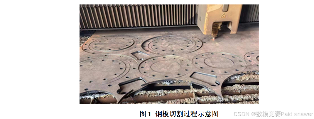
  注：(1) 空程是指在切割设备所进行的一系列操作中不产生切割效果的水平运动路径(垂直运动路径不计入空程)；(2) 本题默认切割起始点均为右下角点(见各图所示)；(3) 本题下料切割布局图中的实线均为切割线。
  请查阅相关资料，完成下列四个切割任务N1~N4：
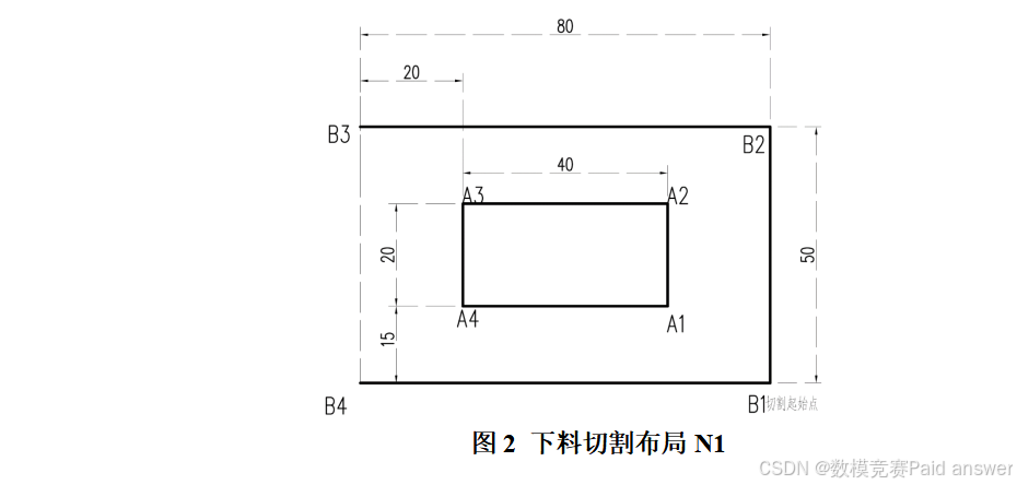
  问题1：给定如图2所示的下料切割布局N1，其中B3-B4为钢板边界线，不用切割，B1为切割起始点。请建立数学模型，设计最优切割路径方案，并给出最优切割路径的空程总长度。

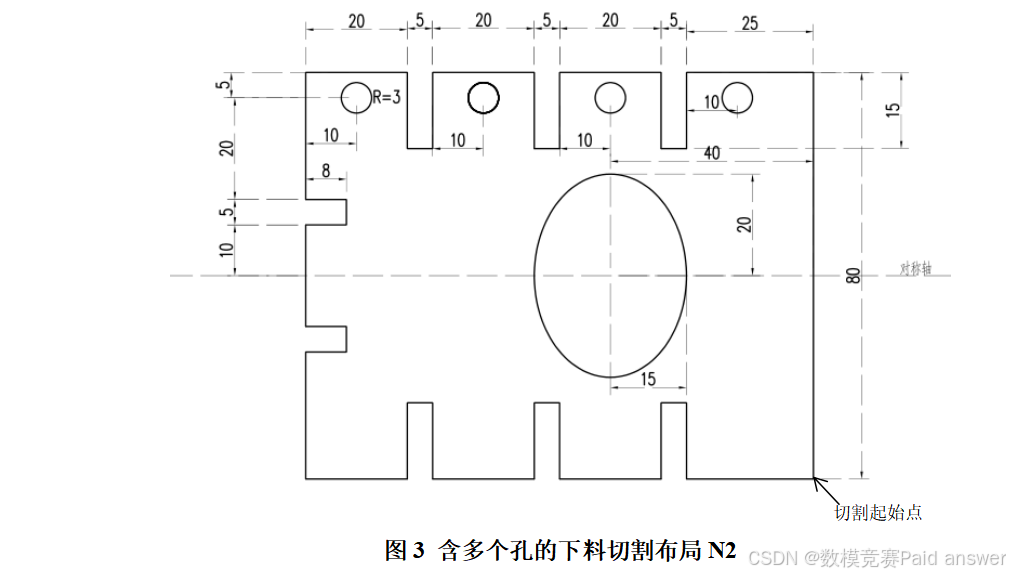
  问题2：给定下料切割布局N2见图3，构件的外边界切割成上下对称的锯齿状，同时内部切割出四个半径为3的圆形和一个椭圆形。请根据下料切割布局N2的参数信息，建立数学模型，设计最优切割路径方案，并给出最优切割路径的空程总长度。

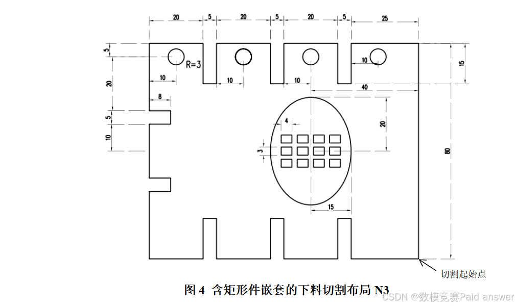
  问题3：给定下料切割布局N3见图4。N3与N2相比，需要在椭圆中多切割出12个矩形件(它们在椭圆中的位置是对称分布的，左右相邻的两个矩形件的中心距离为6，上下相邻的两个矩形件的中心距离为5)。请建立数学模型，设计最优切割路径方案，并给出最优切割路径的空程总长度(要求椭圆内部的所有矩形件要先于椭圆切割)。

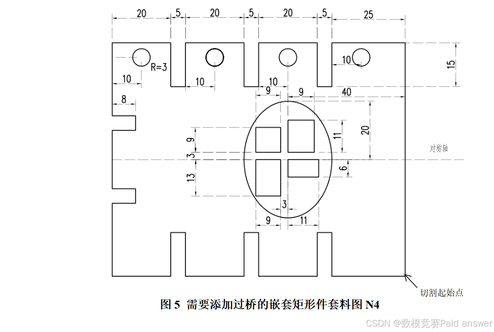
  问题4：给定下料切割布局N4见图5，需要在椭圆中切割出4个矩形小零件。由于小零件尺寸较小，为防止小零件掉落，两个相邻的小零件之间需要采用“过桥”的方式，使得相邻零件连接成一个大尺寸零件，要求“过桥”与矩形小零件顶点的最短距离至少为1。“过桥”的宽度为2，且在空程计算中不可以忽略“过桥”的宽度。
  请根据N4的具体情况，建立数学模型，确定“过桥”的数目和位置，设计最优切割路径方案，给出最优切割路径的空程总长度(要求切割起始点设计在钢板的右下角，N4中的小圆形切割件不考虑过桥问题)。

整体求解过程概述(摘要)

  针对问题一，为了探究开放外轮廓与内矩形之间的最短非切割衔接方式，首先将题图坐标化为开放折线与闭合矩形两类必切割对象，并基于三角不等式建立解析几何模型。通过证明最优衔接点必位于内矩形左边界的纵向中点，得到切割顺序“B1—B2—B3、经Q点切割内矩形、B4—B1”，最小空程为 64.0312。候选顶点方案与解析下界对照表明，该结果满足全局最优性。
  针对问题二，鉴于四个圆孔和椭圆均位于锯齿外轮廓内部，引入“外轮廓主干—内轮廓往返插入”策略，将外轮廓视作零空程切割主干。首先进行几何数据理解、轮廓间最短距离矩阵分析与曲线离散精度检验，再分别计算四个圆孔及椭圆至外轮廓的最短欧氏距离。由此可得四个圆孔的单程插入距离均为2，椭圆的单程插入距离为 3.6519，最小总空程为 23.3038。高分辨率离散收敛结果验证了计算稳定性。
  针对问题三，在问题二几何模型的基础上进一步考虑12个嵌套矩形及“全部矩形先于椭圆”的偏序约束。考虑到访问顺序与连续落刀点同时决定空程，引入连续旅行商邻域思想，构建“外轮廓接入点—矩形序列—椭圆落刀点—外轮廓返回点”的闭合插入模型。采用多起点构造生成候选序列，利用分层动态规划精确求解固定序列下的最优落刀点，并以交换邻域和2-opt进行序列改进。最终矩形访问次序为 3—2—1—5—9—10—6—7—11—12—8—4，嵌套模块空程为 70.4065，计入四圆插入后总空程为 86.4065。方法比较、离散敏感性和随机定位扰动验证表明结果具有较好的合理性与鲁棒性。
  针对问题四，为了在防止小零件掉落的同时降低空程，将四个矩形小零件抽象为邻接图。由连通图的生成树性质可知，连接4个零件至少需要3座桥，因而采用“左下—左上、左上—右上、右上—右下”的三桥方案。随后对桥宽2和顶点净距不小于1的约束进行几何核验，并将过桥宽度引起的三次非切割跨越纳入目标函数。最终四圆往返、外轮廓—椭圆往返、椭圆—组合件往返及桥宽贡献之和为 30.6641。桥数对比与桥宽灵敏度分析表明三桥方案在可行性和经济性之间达到平衡。
  综上，本文按照“数据理解与探索—几何预处理—特征工程—模型构建—算法求解—误差评估—工程解释”的技术路线，形成了解析几何模型、主干插入模型、带偏序约束的连续邻域路径模型与过桥生成树模型。模型既保留了题目几何结构和工艺顺序，又通过多方法比较、离散收敛与鲁棒性检验控制泛化误差，可推广至多轮廓激光切割、数控冲裁和具有嵌套优先级的二维加工路径规划。

模型假设：

  假设1：切割头在平面内的空程按两点间欧氏距离计量，忽略加速、减速和转弯半径对路径长度的二阶影响。
  假设2：切割线本身的运动不计入目标函数；切割头抬升和下降的竖直位移不计入空程。
  假设3：每个闭合轮廓可在任意边界点落刀，完成一周切割后回到同一落刀点。
  假设4：外轮廓可在切割过程中暂停，并在同一位置完成内轮廓往返插入后继续切割；暂停本身不产生额外距离。
  假设5：N3中全部12个矩形轮廓必须完整切割后方可开始椭圆轮廓切割；圆孔与外轮廓之间不存在额外顺序限制。
  假设6：题图的线宽仅用于显示，不代表几何宽度；所有坐标以尺寸标注为准，图像像素只用于辅助判断相对位置。
  假设7：N4的过桥为宽度2的未切材料连接区，切割头跨越桥宽时激光关闭，因而每座桥对应2个长度单位的空程贡献。
  假设8：忽略热变形、割缝补偿、穿孔时间和材料翘曲；这些因素在模型推广部分作为扩展变量讨论。

问题分析：

  问题一问题分析
  针对 N1 单外框搭配内置矩形的钢板切割布局，本题属于简单平面几何最短路径优化问题，核心目标是求解切割头最小空程移动长度。题目限定外框 B3-B4 为无需切割的钢板原生边界，切割起点固定在 B1，仅存在一条开放折线外轮廓与单个闭合内矩形两类待切割线条，两类轮廓之间必须存在抬刀空程转移。利用图形上下对称几何特性可采用反射解析法直接推导最优衔接点位，无需复杂遍历算法；建模核心是构建两点间距离和最小化目标函数，对比多种候选落刀方案验证解析解全局最优性，最终输出完整切割顺序与最小空程数值。
  问题二问题分析
  针对 N2 带锯齿外轮廓、四圆孔与单椭圆的复合切割布局，本题属于主干往返插入型路径优化问题，承接问题一几何距离计算逻辑。外轮廓可作为无空程切割主干，圆孔、椭圆均为独立闭合内轮廓，完成单轮廓切割需往返外轮廓形成两段空程；圆孔坐标规整可直接解析最短接入距离，椭圆为曲线轮廓需采用离散采样法求解轮廓间最小欧氏距离。难点在于判断内轮廓串联与单独往返的成本差异，通过轮廓距离矩阵证明单独插入更节省空程，同时设置多组离散采样精度完成数值收敛检验，保证计算结果稳定可靠。
  问题三问题分析
  针对 N2 基础上新增 12 个嵌套矩形、附带 “全部矩形优先于椭圆切割” 工艺偏序约束的布局，本题为带顺序限制的连续旅行商优化问题。模型分为双层求解结构：外层优化矩形访问排列顺序，内层利用分层动态规划求解固定序列下各矩形最优落刀点；初始采用蛇形、最近邻多类序列构造方案，搭配 2-opt 局部搜索迭代降低总转移空程。需严格遵循矩形切割前置约束，不可打乱矩形与椭圆加工次序，同时通过离散精度测试、坐标扰动鲁棒性实验验证最优序列稳定性，叠加问题二圆孔往返空程得到整体最小空程总长。
  问题四问题分析
  针对椭圆内部四块需过桥连接的小型矩形零件布局，本题融合图论连通性约束与几何距离优化双重内容。首先利用最小生成树理论判定连通四块零件最少需要 3 座过桥，2 桥方案无法满足零件不掉落工艺要求，4 桥会产生冗余空程；其次建立过桥几何约束模型，核验桥宽 2、桥与零件顶点净距不小于 1 的硬性条件；最后整合四圆孔往返、椭圆接入、过桥跨越、组合件与椭圆转移四类空程分量构建总目标函数，通过过桥数量、桥宽灵敏度分析对比不同方案经济性，输出满足全部几何与工艺约束的最小空程结果。

模型的建立与求解整体论文缩略图

全部论文请见下方“ 只会建模 QQ名片” 点击QQ名片即可

程序代码：

from __future__ import annotations

import argparse
import json
import math
import random
from dataclasses import dataclass
from pathlib import Path
from typing import Dict, Iterable, List, Sequence, Tuple

import matplotlib
matplotlib.use("Agg")
import matplotlib.pyplot as plt
from matplotlib import font_manager
from matplotlib.patches import Circle, Ellipse, Polygon, Rectangle
import networkx as nx
import numpy as np
import pandas as pd
from scipy.spatial.distance import cdist
from scipy.stats import gaussian_kde, kurtosis, skew

Point = Tuple[float, float]

# —————————————————————————–
# 0. 绘图与通用工具
# —————————————————————————–
def configure_chinese_font() –> str:
"""注册中文字体，避免标题、图例和坐标轴出现方框。"""
candidates = [
"/usr/share/fonts/opentype/noto/NotoSansCJK-Regular.ttc",
"/usr/share/fonts/opentype/noto/NotoSansCJK-Bold.ttc",
"/usr/share/fonts/truetype/arphic-gbsn00lp/gbsn00lp.ttf",
]
selected = None
for path in candidates:
if Path(path).exists():
font_manager.fontManager.addfont(path)
selected = font_manager.FontProperties(fname=path).get_name()
break
if selected is None:
for name in ["Noto Sans CJK SC", "SimHei", "Microsoft YaHei", "Arial Unicode MS"]:
try:
font_manager.findfont(name, fallback_to_default=False)
selected = name
break
except Exception:
continue
if selected is None:
raise RuntimeError("未检测到可用中文字体，请安装 Noto Sans CJK SC 后重试。")
plt.rcParams.update({
"font.family": selected,
"font.sans-serif": [selected],
"axes.unicode_minus": False,
"figure.dpi": 130,
"savefig.dpi": 220,
"axes.titlesize": 12,
"axes.labelsize": 10,
"legend.fontsize": 9,
})
return selected

def euclidean(a: np.ndarray, b: np.ndarray) –> float:
return float(np.linalg.norm(a – b))

def savefig(path: Path) –> None:
path.parent.mkdir(parents=True, exist_ok=True)
plt.tight_layout()
plt.savefig(path, bbox_inches="tight")
plt.close()

def sample_polyline(vertices: Sequence[Point], n_per_segment: int = 20,
closed: bool = True) –> np.ndarray:
pts: List[np.ndarray] = []
n_seg = len(vertices) if closed else len(vertices) – 1
for i in range(n_seg):
a = np.asarray(vertices[i], dtype=float)
b = np.asarray(vertices[(i + 1) % len(vertices)], dtype=float)
for t in np.linspace(0, 1, n_per_segment, endpoint=False):
pts.append(a + t * (b – a))
if not closed:
pts.append(np.asarray(vertices[–1], dtype=float))
return np.asarray(pts)

def sample_rectangle(x1: float, y1: float, x2: float, y2: float,
n_per_side: int = 16) –> np.ndarray:
return sample_polyline([(x1, y1), (x2, y1), (x2, y2), (x1, y2)],
n_per_side, True)

def sample_circle(cx: float, cy: float, r: float, n: int = 360) –> np.ndarray:
theta = np.linspace(0, 2 * np.pi, n, endpoint=False)
return np.column_stack([cx + r * np.cos(theta), cy + r * np.sin(theta)])

def sample_ellipse(cx: float, cy: float, rx: float, ry: float,
n: int = 720) –> np.ndarray:
theta = np.linspace(0, 2 * np.pi, n, endpoint=False)
return np.column_stack([cx + rx * np.cos(theta), cy + ry * np.sin(theta)])

def minimum_distance(a: np.ndarray, b: np.ndarray) –> Tuple[float, np.ndarray, np.ndarray]:
dist = cdist(a, b)
i, j = np.unravel_index(np.argmin(dist), dist.shape)
return float(dist[i, j]), a[i].copy(), b[j].copy()

def polyline_length(vertices: Sequence[Point], closed: bool = True) –> float:
arr = np.asarray(vertices, dtype=float)
if closed:
arr = np.vstack([arr, arr[0]])
return float(np.linalg.norm(np.diff(arr, axis=0), axis=1).sum())

def ellipse_perimeter_ramanujan(a: float, b: float) –> float:
h = ((a – b) / (a + b)) ** 2
return math.pi * (a + b) * (1 + 3 * h / (10 + math.sqrt(4 – 3 * h)))

# —————————————————————————–
# 1. 几何数据定义
# —————————————————————————–
OUTER_VERTICES: List[Point] = [
(0, 0), (20, 0), (20, 20), (25, 20), (25, 0),
(45, 0), (45, 20), (50, 20), (50, 0),
(70, 0), (70, 20), (75, 20), (75, 0),
(100, 0), (100, 80),
(75, 80), (75, 60), (70, 60), (70, 80),
(50, 80), (50, 60), (45, 60), (45, 80),
(25, 80), (25, 60), (20, 60), (20, 80),
(0, 80), (0, 55), (8, 55), (8, 50),
(0, 50), (0, 30), (8, 30), (8, 25), (0, 25),
]
START_N234 = np.array([100.0, 0.0])
ELLIPSE_PARAM = (60.0, 40.0, 15.0, 20.0)
CIRCLE_CENTERS = [(10.0, 75.0), (35.0, 75.0), (60.0, 75.0), (85.0, 75.0)]

# N3: 图示为4列×3行，矩形尺寸4×3，横向中心距6、纵向中心距5。
N3_CENTERS = [(x, y) for y in (35.0, 40.0, 45.0) for x in (51.0, 57.0, 63.0, 69.0)]

# N4: 依据图中尺寸与对称轴进行矢量化重建。三个桥组成生成树：
# 左下—左上、左上—右上、右上—右下。
N4_RECTS = {
"左上件": (48.5, 42.5, 57.5, 51.5),
"右上件": (60.5, 42.5, 69.5, 51.5),
"左下件": (51.5, 28.5, 57.5, 39.5),
"右下件": (60.5, 30.5, 71.5, 39.5),
}
N4_BRIDGES = {
"桥1（左列竖向）": (54.5, 39.5, 56.5, 42.5),
"桥2（上排横向）": (57.5, 46.0, 60.5, 48.0),
"桥3（右列竖向）": (64.0, 39.5, 66.0, 42.5),
}

@dataclass
class ModelResults:
n1_length: float
n2_length: float
n3_length: float
n4_length: float
n3_order: List[int]
n3_nested_length: float
outer_ellipse_distance: float
circle_outer_distances: List[float]
ellipse_bridge_distance: float

# —————————————————————————–
# 2. 数据理解与统计
# —————————————————————————–
def build_geometric_feature_table() –> pd.DataFrame:
rows = [
{"布局": "N1", "对象": "外轮廓可切线", "类型": "开放折线", "数量": 1,
"周长或线长": 80 + 50 + 80, "面积": np.nan},
{"布局": "N1", "对象": "内矩形", "类型": "矩形", "数量": 1,
"周长或线长": 2 * (40 + 20), "面积": 40 * 20},
{"布局": "N2", "对象": "锯齿外轮廓", "类型": "多边形", "数量": 1,
"周长或线长": polyline_length(OUTER_VERTICES), "面积": np.nan},
{"布局": "N2", "对象": "圆孔", "类型": "圆", "数量": 4,
"周长或线长": 2 * math.pi * 3, "面积": math.pi * 3 ** 2},
{"布局": "N2", "对象": "椭圆孔", "类型": "椭圆", "数量": 1,
"周长或线长": ellipse_perimeter_ramanujan(15, 20), "面积": math.pi * 15 * 20},
{"布局": "N3", "对象": "嵌套矩形", "类型": "矩形", "数量": 12,
"周长或线长": 2 * (4 + 3), "面积": 4 * 3},
{"布局": "N4", "对象": "过桥小件", "类型": "异形组合", "数量": 4,
"周长或线长": np.mean([2 * ((x2 – x1) + (y2 – y1)) for x1, y1, x2, y2 in N4_RECTS.values()]),
"面积": np.mean([(x2 – x1) * (y2 – y1) for x1, y1, x2, y2 in N4_RECTS.values()])},
]
return pd.DataFrame(rows)

def descriptive_statistics(values: Sequence[float], name: str) –> Dict[str, float]:
arr = np.asarray(values, dtype=float)
return {
"指标": name,
"样本数": int(arr.size),
"均值": float(np.mean(arr)),
"标准差": float(np.std(arr, ddof=1)) if arr.size > 1 else 0.0,
"变异系数": float(np.std(arr, ddof=1) / np.mean(arr)) if arr.size > 1 and np.mean(arr) != 0 else 0.0,
"最小值": float(np.min(arr)),
"中位数": float(np.median(arr)),
"最大值": float(np.max(arr)),
"偏度": float(skew(arr, bias=False)) if arr.size >= 3 else 0.0,
"峰度": float(kurtosis(arr, fisher=True, bias=False)) if arr.size >= 4 else 0.0,
}

# —————————————————————————–
# 3. 问题1解析模型
# —————————————————————————–
def solve_n1() –> Tuple[float, List[np.ndarray]]:
b3 = np.array([0.0, 50.0])
b4 = np.array([0.0, 0.0])
q = np.array([20.0, 25.0])
length = euclidean(b3, q) + euclidean(q, b4)
# 切割顺序：B1-B2-B3；空程至Q；切内矩形一周；空程至B4；切B4-B1。
route = [np.array([80.0, 0.0]), np.array([80.0, 50.0]), b3, q, b4, np.array([80.0, 0.0])]
return length, route

# —————————————————————————–
# 4. 问题2主干插入模型
# —————————————————————————–
def solve_n2(resolution: int = 720) –> Tuple[float, Dict[str, Tuple[float, np.ndarray, np.ndarray]]]:
outer = sample_polyline(OUTER_VERTICES, max(8, resolution // 36), True)
ellipse = sample_ellipse(*ELLIPSE_PARAM, n=resolution)
details: Dict[str, Tuple[float, np.ndarray, np.ndarray]] = {}
for i, (cx, cy) in enumerate(CIRCLE_CENTERS, 1):
# 四个圆孔的圆心均位于y=75，半径为3，正上方外轮廓为y=80，
# 因而最短距离可解析得到 80-(75+3)=2，避免离散采样误差。
details[f"圆孔C{i}"] = (2.0, np.array([cx, 80.0]), np.array([cx, 78.0]))
details["椭圆E"] = minimum_distance(outer, ellipse)
total = 2.0 * sum(v[0] for v in details.values())
return total, details

# —————————————————————————–
# 5. 问题3：固定顺序的分层动态规划 + 2-opt
# —————————————————————————–
class N3Optimizer:
def __init__(self, outer_seg_samples: int = 10, rect_side_samples: int = 16,
ellipse_samples: int = 300):
self.outer = sample_polyline(OUTER_VERTICES, outer_seg_samples, True)
self.ellipse = sample_ellipse(*ELLIPSE_PARAM, n=ellipse_samples)
self.rects = [sample_rectangle(x – 2, y – 1.5, x + 2, y + 1.5,
rect_side_samples) for x, y in N3_CENTERS]
self.d_or = [cdist(self.outer, r) for r in self.rects]
self.d_re = [cdist(r, self.ellipse) for r in self.rects]
self.d_eo = cdist(self.ellipse, self.outer)
self.d_rr = {(i, j): cdist(self.rects[i], self.rects[j])
for i in range(12) for j in range(12) if i != j}
self.eval_counter = 0

def evaluate_order(self, order: Sequence[int], return_path: bool = False):
self.eval_counter += 1
dp = self.d_or[order[0]].copy() # 外轮廓采样点 × 第一个矩形采样点
backpointers: List[np.ndarray] = []
for a, b in zip(order[:–1], order[1:]):
value = dp[:, :, None] + self.d_rr[(a, b)][None, :, :]
if return_path:
backpointers.append(np.argmin(value, axis=1))
dp = np.min(value, axis=1)
value_e = dp[:, :, None] + self.d_re[order[–1]][None, :, :]
bp_e = np.argmin(value_e, axis=1)
dp_e = np.min(value_e, axis=1)
total = dp_e + self.d_eo.T
oi, ei = np.unravel_index(np.argmin(total), total.shape)
best = float(total[oi, ei])
if not return_path:
return best
idx = int(bp_e[oi, ei])
rect_indices = [0] * len(order)
rect_indices[–1] = idx
for t in range(len(order) – 2, –1, –1):
idx = int(backpointers[t][oi, idx])
rect_indices[t] = idx
points = [self.outer[oi]]
points.extend(self.rects[order[k]][rect_indices[k]] for k in range(len(order)))
points.extend([self.ellipse[ei], self.outer[oi]])
return best, points, int(oi), int(ei), rect_indices

@staticmethod
def initial_orders(seed: int = 2024) –> List[List[int]]:
rng = random.Random(seed)
grid = np.arange(12).reshape(3, 4)
candidates: List[List[int]] = []
# 行蛇形与列蛇形
for reverse_rows in (False, True):
rows = list(range(3))[::–1] if reverse_rows else list(range(3))
for phase in (0, 1):
order: List[int] = []
for k, r in enumerate(rows):
cols = list(range(4))
if (k + phase) % 2:
cols.reverse()
order.extend(int(grid[r, c]) for c in cols)
candidates.extend([order, order[::–1]])
for reverse_cols in (False, True):
cols = list(range(4))[::–1] if reverse_cols else list(range(4))
for phase in (0, 1):
order = []
for k, c in enumerate(cols):
rows = list(range(3))
if (k + phase) % 2:
rows.reverse()
order.extend(int(grid[r, c]) for r in rows)
candidates.extend([order, order[::–1]])
# 基于中心距离的扰动最近邻
centers = np.asarray(N3_CENTERS)
center_dist = cdist(centers, centers)
for start in range(12):
for noise_level in range(2):
remaining = set(range(12))
remaining.remove(start)
order = [start]
while remaining:
cur = order[–1]
nxt = min(remaining,
key=lambda j: center_dist[cur, j] + rng.random() * 0.08 * noise_level)
order.append(nxt)
remaining.remove(nxt)
candidates.extend([order, order[::–1]])
candidates.append([3, 7, 11, 10, 6, 5, 9, 8, 4, 0, 1, 2])
candidates.append([2, 1, 0, 4, 8, 9, 5, 6, 10, 11, 7, 3])
unique = {tuple(x): x for x in candidates}
return list(unique.values())

def solve(self) –> Tuple[float, List[int], List[np.ndarray], pd.DataFrame]:
history: List[Dict[str, float]] = []
best_value = math.inf
best_order: List[int] = []
for i, order in enumerate(self.initial_orders()):
value = self.evaluate_order(order)
if value < best_value:
best_value, best_order = value, order.copy()
history.append({"评价次数": self.eval_counter, "当前最优": best_value,
"阶段": "多起点构造"})
# 交换与2-opt复合邻域
improved = True
iteration = 0
while improved and iteration < 2:
improved = False
iteration += 1
incumbent = best_order.copy()
for i in range(12):
for j in range(i + 1, 12):
trial = incumbent.copy()
trial[i], trial[j] = trial[j], trial[i]
value = self.evaluate_order(trial)
if value < best_value – 1e-9:
best_value, best_order, improved = value, trial, True
history.append({"评价次数": self.eval_counter, "当前最优": best_value,
"阶段": "交换邻域"})
trial = incumbent[:i] + list(reversed(incumbent[i:j + 1])) + incumbent[j + 1:]
value = self.evaluate_order(trial)
if value < best_value – 1e-9:
best_value, best_order, improved = value, trial, True
history.append({"评价次数": self.eval_counter, "当前最优": best_value,
"阶段": "2-opt邻域"})
if improved:
continue
best_value, points, *_ = self.evaluate_order(best_order, return_path=True)
return best_value, best_order, points, pd.DataFrame(history)

# —————————————————————————–
# 6. 问题4：桥数与位置模型
# —————————————————————————–
def n4_adjacency_graph() –> nx.Graph:
graph = nx.Graph()
graph.add_nodes_from(N4_RECTS.keys())
graph.add_edge("左下件", "左上件", name="桥1", width=2.0)
graph.add_edge("左上件", "右上件", name="桥2", width=2.0)
graph.add_edge("右上件", "右下件", name="桥3", width=2.0)
# 其余候选邻接边可作为替代方案，权重略大。
graph.add_edge("左下件", "右下件", name="候选桥4", width=2.0, candidate=True)
return graph

def bridge_clearance(bridge: Tuple[float, float, float, float],
rects: Iterable[Tuple[float, float, float, float]]) –> float:
x1, y1, x2, y2 = bridge
corners = []
for a, b, c, d in rects:
corners.extend([(a, b), (a, d), (c, b), (c, d)])
# 桥中心线段端部与所有矩形顶点之间的保守最短距离。
sample = sample_rectangle(x1, y1, x2, y2, 30)
return float(min(np.linalg.norm(sample – np.asarray(c), axis=1).min() for c in corners))

def solve_n4(n2_details: Dict[str, Tuple[float, np.ndarray, np.ndarray]]) –> Tuple[float, Dict[str, float]]:
outer_ellipse = n2_details["椭圆E"][0]
ellipse = sample_ellipse(*ELLIPSE_PARAM, n=1200)
rect_samples = {name: sample_rectangle(*rect, n_per_side=50)
for name, rect in N4_RECTS.items()}
ellipse_to_piece = min(minimum_distance(ellipse, pts)[0] for pts in rect_samples.values())
circle_roundtrips = 2 * sum(n2_details[f"圆孔C{i}"][0] for i in range(1, 5))
# 三座宽度为2的桥在切割轨迹中对应三次激光关闭跨越，故计入6个长度单位。
bridge_air = sum((x2 – x1) if (x2 – x1) < (y2 – y1) else (y2 – y1)
for x1, y1, x2, y2 in N4_BRIDGES.values())
total = circle_roundtrips + 2 * outer_ellipse + 2 * ellipse_to_piece + bridge_air
details = {
"四圆往返空程": circle_roundtrips,
"外轮廓—椭圆往返": 2 * outer_ellipse,
"椭圆—过桥组合件往返": 2 * ellipse_to_piece,
"三座过桥跨越空程": bridge_air,
"椭圆—组合件最短距离": ellipse_to_piece,
}
return total, details

# —————————————————————————–
# 7. 可视化
# —————————————————————————–
def draw_outer(ax, lw: float = 1.6, label: str | None = None):
arr = np.asarray(OUTER_VERTICES + [OUTER_VERTICES[0]])
ax.plot(arr[:, 0], arr[:, 1], linewidth=lw, label=label)

def standard_axes(ax, title: str):
ax.set_aspect("equal", adjustable="box")
ax.set_xlim(–5, 105)
ax.set_ylim(–5, 85)
ax.set_xlabel("x 坐标")
ax.set_ylabel("y 坐标")
ax.set_title(title)
ax.grid(alpha=0.18)

def plot_workflow(out: Path):
fig, ax = plt.subplots(figsize=(11, 3.5))
ax.axis("off")
labels = ["题图尺寸解析", "几何拓扑重建", "统计探索与可视化", "路径优化建模",
"算法求解与收敛", "可行性和鲁棒性验证", "工程决策输出"]
xs = np.linspace(0.06, 0.94, len(labels))
for i, (x, text) in enumerate(zip(xs, labels)):
ax.text(x, 0.55, text, ha="center", va="center",
bbox=dict(boxstyle="round,pad=0.45", facecolor="white", edgecolor="0.35"),
transform=ax.transAxes)
if i < len(labels) – 1:
ax.annotate("", xy=(xs[i + 1] – 0.065, 0.55), xytext=(x + 0.065, 0.55),
arrowprops=dict(arrowstyle="->", lw=1.4), xycoords=ax.transAxes)
ax.text(0.5, 0.16, "数据理解与探索 → 数据预处理 → 特征工程 → 模型构建 → 训练与评估 → 结果解释",
ha="center", transform=ax.transAxes)
savefig(out / "fig01_workflow.png")

def plot_layouts(out: Path):
# N1
fig, ax = plt.subplots(figsize=(8, 5.2))
outer = np.array([[0, 50], [80, 50], [80, 0], [0, 0]])
ax.plot([0, 80, 80, 0], [50, 50, 0, 0], lw=2)
ax.add_patch(Rectangle((20, 15), 40, 20, fill=False, lw=2))
for p, text in [((80, 0), "B1 起点"), ((80, 50), "B2"), ((0, 50), "B3"), ((0, 0), "B4")]:
ax.scatter(*p, s=28); ax.text(p[0] + 1, p[1] + 1, text)
ax.text(2, 24, "B3—B4 为钢板边界线\\n不实施切割", va="center")
ax.set_aspect("equal"); ax.set_xlim(–5, 85); ax.set_ylim(–5, 55)
ax.set_xlabel("x 坐标"); ax.set_ylabel("y 坐标"); ax.set_title("N1 坐标化重建结果")
ax.grid(alpha=.2)
savefig(out / "fig02_layout_n1.png")

# N2
fig, ax = plt.subplots(figsize=(9, 6.5))
draw_outer(ax)
for i, (x, y) in enumerate(CIRCLE_CENTERS, 1):
ax.add_patch(Circle((x, y), 3, fill=False, lw=1.5)); ax.text(x, y, f"C{i}", ha="center", va="center")
ax.add_patch(Ellipse((60, 40), 30, 40, fill=False, lw=1.6)); ax.text(60, 40, "E", ha="center")
ax.scatter(*START_N234, s=45, marker="*"); ax.annotate("切割起点", START_N234, xytext=(82, 6),
arrowprops=dict(arrowstyle="->"))
standard_axes(ax, "N2 多孔锯齿构件的矢量化布局")
savefig(out / "fig03_layout_n2.png")

# N3
fig, ax = plt.subplots(figsize=(9, 6.5))
draw_outer(ax)
for x, y in CIRCLE_CENTERS: ax.add_patch(Circle((x, y), 3, fill=False, lw=1.1))
ax.add_patch(Ellipse((60, 40), 30, 40, fill=False, lw=1.5))
for i, (x, y) in enumerate(N3_CENTERS):
ax.add_patch(Rectangle((x – 2, y – 1.5), 4, 3, fill=False, lw=1.2))
ax.text(x, y, str(i + 1), ha="center", va="center", fontsize=7)
standard_axes(ax, "N3 含12个嵌套矩形的布局重建")
savefig(out / "fig04_layout_n3.png")

# N4
fig, ax = plt.subplots(figsize=(9, 6.5))
draw_outer(ax)
for x, y in CIRCLE_CENTERS: ax.add_patch(Circle((x, y), 3, fill=False, lw=1.1))
ax.add_patch(Ellipse((60, 40), 30, 40, fill=False, lw=1.5))
for name, (x1, y1, x2, y2) in N4_RECTS.items():
ax.add_patch(Rectangle((x1, y1), x2 – x1, y2 – y1, fill=False, lw=1.4))
ax.text((x1 + x2) / 2, (y1 + y2) / 2, name, ha="center", va="center", fontsize=7)
for name, (x1, y1, x2, y2) in N4_BRIDGES.items():
ax.add_patch(Rectangle((x1, y1), x2 – x1, y2 – y1, alpha=0.25, hatch="///"))
standard_axes(ax, "N4 三桥连接方案的几何重建")
savefig(out / "fig05_layout_n4.png")

def plot_feature_statistics(out: Path, feature_df: pd.DataFrame,
pair_values: Sequence[float], stats_df: pd.DataFrame):
expanded = []
for _, r in feature_df.iterrows():
for _ in range(int(r["数量"])):
expanded.append((r["布局"] + "-" + r["对象"], r["周长或线长"]))
labels, vals = zip(*expanded)
fig, ax = plt.subplots(figsize=(10, 6))
y = np.arange(len(vals))
ax.barh(y, vals)
ax.set_yticks(y, labels)
ax.set_xlabel("单个轮廓的周长或有效线长")
ax.set_title("各类切割轮廓几何规模比较")
ax.grid(axis="x", alpha=.2)
savefig(out / "fig06_contour_length_bar.png")

vals_arr = np.asarray(pair_values)
fig, ax = plt.subplots(figsize=(8, 5.2))
ax.hist(vals_arr, bins=16, density=True, alpha=.65, label="直方图")
if len(np.unique(vals_arr)) > 2:
xs = np.linspace(vals_arr.min(), vals_arr.max(), 300)
ax.plot(xs, gaussian_kde(vals_arr)(xs), lw=2, label="核密度估计")
ax.axvline(np.mean(vals_arr), linestyle="–", label=f"均值={np.mean(vals_arr):.2f}")
ax.axvline(np.median(vals_arr), linestyle=":", label=f"中位数={np.median(vals_arr):.2f}")
ax.set_xlabel("轮廓间最短欧氏距离")
ax.set_ylabel("概率密度")
ax.set_title("几何转移距离的分布形态")
ax.legend()
savefig(out / "fig07_distance_hist_kde.png")

fig, ax = plt.subplots(figsize=(8, 5))
sorted_v = np.sort(vals_arr)
ecdf = np.arange(1, len(sorted_v) + 1) / len(sorted_v)
ax.step(sorted_v, ecdf, where="post")
for q in (0.25, 0.5, 0.75):
value = np.quantile(vals_arr, q)
ax.axvline(value, linestyle="–", alpha=.55)
ax.text(value, q, f"Q{int(q*100)}={value:.2f}", rotation=90, va="bottom")
ax.set_xlabel("轮廓间最短距离")
ax.set_ylabel("经验累积分布")
ax.set_title("轮廓间距离的ECDF及四分位结构")
ax.grid(alpha=.2)
savefig(out / "fig08_distance_ecdf.png")

fig, ax = plt.subplots(figsize=(9, 4.8))
cols = ["均值", "标准差", "变异系数", "偏度", "峰度"]
matrix = stats_df.set_index("指标")[cols].to_numpy(dtype=float)
image = ax.imshow(matrix, aspect="auto")
ax.set_xticks(range(len(cols)), cols)
ax.set_yticks(range(len(stats_df)), stats_df["指标"])
for i in range(matrix.shape[0]):
for j in range(matrix.shape[1]):
ax.text(j, i, f"{matrix[i,j]:.2f}", ha="center", va="center", fontsize=8)
plt.colorbar(image, ax=ax, label="标准化前统计量")
ax.set_title("描述性统计、偏度与峰度指标矩阵")
savefig(out / "fig09_stats_heatmap.png")

def plot_n1(out: Path, result: float, route: List[np.ndarray]):
fig, ax = plt.subplots(figsize=(8, 5.2))
ax.plot([0, 80, 80, 0], [50, 50, 0, 0], lw=2, label="切割线")
ax.add_patch(Rectangle((20, 15), 40, 20, fill=False, lw=2))
# 空程只画 B3-Q-B4
p = np.vstack([route[2], route[3], route[4]])
ax.plot(p[:, 0], p[:, 1], linestyle="–", marker="o", lw=2, label="空程")
ax.annotate(f"Q=(20,25)\\n总空程={result:.3f}", route[3], xytext=(35, 43),
arrowprops=dict(arrowstyle="->"))
ax.set_aspect("equal"); ax.set_xlim(–5, 85); ax.set_ylim(–5, 55)
ax.set_xlabel("x 坐标"); ax.set_ylabel("y 坐标"); ax.set_title("N1 解析最优切割路径")
ax.legend(); ax.grid(alpha=.2)
savefig(out / "fig10_n1_optimal_route.png")

alternatives = {
"经内矩形左边中点": result,
"经内矩形左下角": math.dist((0, 50), (20, 15)) + math.dist((20, 15), (0, 0)),
"经内矩形左上角": math.dist((0, 50), (20, 35)) + math.dist((20, 35), (0, 0)),
"直接B3到B4后再访问内框": 50 + 15,
}
fig, ax = plt.subplots(figsize=(8, 4.8))
ax.bar(alternatives.keys(), alternatives.values())
ax.set_ylabel("空程长度")
ax.set_title("N1 候选衔接点方案比较")
ax.tick_params(axis="x", rotation=18)
for i, v in enumerate(alternatives.values()): ax.text(i, v + .6, f"{v:.2f}", ha="center")
savefig(out / "fig11_n1_alternative_compare.png")

def plot_n2(out: Path, details: Dict[str, Tuple[float, np.ndarray, np.ndarray]], total: float):
names = list(details)
values = [details[n][0] for n in names]
fig, ax = plt.subplots(figsize=(8.5, 4.8))
ax.stem(names, values, basefmt=" ")
ax.set_ylabel("至外轮廓的最短距离")
ax.set_title("N2 各内轮廓的最短插入距离")
for i, v in enumerate(values): ax.text(i, v + .12, f"{v:.3f}", ha="center")
savefig(out / "fig12_n2_min_distance_lollipop.png")

fig, ax = plt.subplots(figsize=(9, 6.5))
draw_outer(ax, label="锯齿外轮廓（主干）")
for i, (cx, cy) in enumerate(CIRCLE_CENTERS, 1):
ax.add_patch(Circle((cx, cy), 3, fill=False, lw=1.4))
a, b = details[f"圆孔C{i}"][1], details[f"圆孔C{i}"][2]
ax.plot([a[0], b[0]], [a[1], b[1]], "–", lw=1.8)
ax.add_patch(Ellipse((60, 40), 30, 40, fill=False, lw=1.6))
a, b = details["椭圆E"][1], details["椭圆E"][2]
ax.plot([a[0], b[0]], [a[1], b[1]], "–", lw=2)
ax.text(55, 7, f"主干往返插入总空程 = {total:.3f}")
standard_axes(ax, "N2 最优往返插入位置与路径")
ax.legend(loc="lower left")
savefig(out / "fig13_n2_optimal_route.png")

resolutions = [90, 180, 360, 720, 1080]
vals = [solve_n2(r)[0] for r in resolutions]
fig, ax = plt.subplots(figsize=(8, 4.8))
ax.plot(resolutions, vals, marker="o")
ax.axhline(vals[–1], linestyle="–", label=f"高分辨率基准={vals[–1]:.4f}")
ax.set_xlabel("每条曲线的离散采样规模")
ax.set_ylabel("计算空程长度")
ax.set_title("N2 曲线离散精度的收敛性检验")
ax.legend(); ax.grid(alpha=.2)
savefig(out / "fig14_n2_resolution_convergence.png")

# 距离热图
outer = sample_polyline(OUTER_VERTICES, 12, True)
contours = [sample_circle(x, y, 3, 240) for x, y in CIRCLE_CENTERS]
contours.append(sample_ellipse(*ELLIPSE_PARAM, 400))
contours.append(outer)
labels = ["C1", "C2", "C3", "C4", "椭圆", "外轮廓"]
mat = np.zeros((6, 6))
for i in range(6):
for j in range(i + 1, 6):
mat[i, j] = mat[j, i] = minimum_distance(contours[i], contours[j])[0]
fig, ax = plt.subplots(figsize=(7, 6))
im = ax.imshow(mat)
ax.set_xticks(range(6), labels); ax.set_yticks(range(6), labels)
for i in range(6):
for j in range(6): ax.text(j, i, f"{mat[i,j]:.1f}", ha="center", va="center", fontsize=8)
plt.colorbar(im, ax=ax, label="最短距离")
ax.set_title("N2 轮廓间最短距离矩阵")
savefig(out / "fig15_n2_distance_heatmap.png")

def plot_n3(out: Path, optimizer: N3Optimizer, nested: float, order: List[int],
points: List[np.ndarray], history: pd.DataFrame):
# 先后约束图
fig, ax = plt.subplots(figsize=(10, 4.5))
graph = nx.DiGraph()
graph.add_nodes_from([f"R{i+1}" for i in range(12)], layer=0)
graph.add_node("椭圆E", layer=1)
for i in range(12): graph.add_edge(f"R{i+1}", "椭圆E")
pos = {f"R{i+1}": (i % 6, 1.5 – (i // 6) * 1.0) for i in range(12)}
pos["椭圆E"] = (2.5, –1.0)
nx.draw_networkx(graph, pos, ax=ax, node_size=950, font_size=8, arrowsize=12)
ax.set_title("N3 ‘全部矩形先于椭圆’的偏序约束网络")
ax.axis("off")
savefig(out / "fig16_n3_precedence_dag.png")

fig, ax = plt.subplots(figsize=(8.5, 4.8))
ax.plot(history["评价次数"], history["当前最优"], lw=1.5)
ax.set_xlabel("路径顺序评价次数")
ax.set_ylabel("当前最优嵌套模块空程")
ax.set_title("多起点构造与2-opt搜索的收敛曲线")
ax.grid(alpha=.2)
savefig(out / "fig17_n3_convergence.png")

fig, ax = plt.subplots(figsize=(9, 6.5))
draw_outer(ax)
for x, y in CIRCLE_CENTERS: ax.add_patch(Circle((x, y), 3, fill=False, lw=1.0))
ax.add_patch(Ellipse((60, 40), 30, 40, fill=False, lw=1.4))
for i, (x, y) in enumerate(N3_CENTERS):
ax.add_patch(Rectangle((x – 2, y – 1.5), 4, 3, fill=False, lw=1.2))
ax.text(x, y, f"R{i+1}", ha="center", va="center", fontsize=7)
pp = np.vstack(points)
ax.plot(pp[:, 0], pp[:, 1], "–o", ms=3, lw=1.3, label="嵌套模块空程")
for k, p in enumerate(pp):
if 0 < k < len(pp) – 1:
ax.text(p[0] + .3, p[1] + .3, str(k), fontsize=6)
ax.text(3, 5, f"嵌套模块={nested:.3f}\\n加四圆往返后={nested+16:.3f}")
standard_axes(ax, "N3 严格优先约束下的最优可行路径")
ax.legend(loc="lower left")
savefig(out / "fig18_n3_optimal_route.png")

transitions = np.linalg.norm(np.diff(pp, axis=0), axis=1)
labels = ["外→R" + str(order[0] + 1)]
labels += [f"R{order[i]+1}→R{order[i+1]+1}" for i in range(11)]
labels += [f"R{order[–1]+1}→E", "E→外"]
fig, ax = plt.subplots(figsize=(11, 5.2))
ax.bar(range(len(transitions)), transitions)
ax.set_xticks(range(len(labels)), labels, rotation=65, ha="right")
ax.set_ylabel("空程分段长度")
ax.set_title("N3 最优路径的分段距离贡献")
ax.grid(axis="y", alpha=.2)
savefig(out / "fig19_n3_transition_waterfall.png")

# 多模型对比（同一几何模型，使用不同顺序策略）
candidate_orders = {
"行蛇形": [0,1,2,3,7,6,5,4,8,9,10,11],
"列蛇形": [0,4,8,9,5,1,2,6,10,11,7,3],
"中心最近邻": [3,7,11,10,6,2,1,5,9,8,4,0],
"2-opt优化": order,
}
model_values = {k: optimizer.evaluate_order(v) + 16 for k, v in candidate_orders.items()}
fig, ax = plt.subplots(figsize=(8.5, 4.8))
ax.bar(model_values.keys(), model_values.values())
ax.set_ylabel("总空程长度")
ax.set_title("N3 不同路径构造方法的效果比较")
for i, v in enumerate(model_values.values()): ax.text(i, v + .8, f"{v:.2f}", ha="center")
savefig(out / "fig20_n3_method_compare.png")

# 离散分辨率敏感性
settings = [(4, 80), (6, 120), (8, 180), (12, 240), (16, 300)]
vals = []
for rect_s, ell_s in settings:
opt = N3Optimizer(outer_seg_samples=max(5, rect_s // 2), rect_side_samples=rect_s,
ellipse_samples=ell_s)
vals.append(opt.evaluate_order(order) + 16)
fig, ax = plt.subplots(figsize=(8, 4.8))
x = np.arange(len(settings))
ax.plot(x, vals, marker="o")
ax.set_xticks(x, [f"矩形{a*4}点/椭圆{b}点" for a,b in settings], rotation=20)
ax.set_ylabel("总空程长度")
ax.set_title("N3 离散精度敏感性分析")
ax.grid(alpha=.2)
savefig(out / "fig21_n3_resolution_sensitivity.png")

# 微小加工定位误差的蒙特卡洛近似：固定访问顺序，以中心扰动后的代表点路线衡量变化。
rng = np.random.default_rng(2024)
base_centers = np.asarray([N3_CENTERS[i] for i in order])
samples = []
for _ in range(500):
perturbed = base_centers + rng.normal(0, 0.2, base_centers.shape)
approx = np.linalg.norm(np.diff(perturbed, axis=0), axis=1).sum()
samples.append(approx)
fig, ax = plt.subplots(figsize=(8, 4.8))
ax.boxplot(samples, vert=False, showmeans=True)
ax.set_xlabel("扰动后矩形中心链路长度（代理指标）")
ax.set_yticks([1], ["±0.2定位误差"])
ax.set_title("N3 路径顺序对几何定位误差的鲁棒性")
savefig(out / "fig22_n3_robustness_boxplot.png")

def plot_n4(out: Path, total: float, details: Dict[str, float]):
# 邻接图与最小生成树
graph = n4_adjacency_graph()
mst = nx.minimum_spanning_tree(graph, weight="width")
pos = {"左上件": (0, 1), "右上件": (2, 1), "左下件": (0.5, 0), "右下件": (2.5, 0)}
fig, ax = plt.subplots(figsize=(7.5, 4.5))
nx.draw_networkx_nodes(graph, pos, node_size=1400, ax=ax)
nx.draw_networkx_labels(graph, pos, ax=ax)
nx.draw_networkx_edges(graph, pos, edgelist=list(graph.edges()), style="dashed", width=1, ax=ax)
nx.draw_networkx_edges(mst, pos, edgelist=list(mst.edges()), width=3, ax=ax)
nx.draw_networkx_edge_labels(graph, pos,
edge_labels={(u,v): graph[u][v]["name"] for u,v in graph.edges()},
font_size=8, ax=ax)
ax.set_title("N4 候选邻接关系与3桥最小生成树")
ax.axis("off")
savefig(out / "fig23_n4_mst.png")

# 净距核验
bridge_names = list(N4_BRIDGES)
clearances = [bridge_clearance(N4_BRIDGES[n], N4_RECTS.values()) for n in bridge_names]
fig, ax = plt.subplots(figsize=(8, 4.8))
ax.bar(bridge_names, clearances)
ax.axhline(1.0, linestyle="–", label="题目要求的最小净距1")
ax.set_ylabel("桥边界至矩形顶点的保守最短距离")
ax.set_title("过桥位置的几何可行性检验")
ax.legend(); ax.tick_params(axis="x", rotation=12)
savefig(out / "fig24_n4_clearance.png")

fig, ax = plt.subplots(figsize=(9, 6.5))
draw_outer(ax)
for x, y in CIRCLE_CENTERS: ax.add_patch(Circle((x, y), 3, fill=False, lw=1.0))
ax.add_patch(Ellipse((60, 40), 30, 40, fill=False, lw=1.4))
for name, (x1, y1, x2, y2) in N4_RECTS.items():
ax.add_patch(Rectangle((x1, y1), x2–x1, y2–y1, fill=False, lw=1.3))
for name, (x1, y1, x2, y2) in N4_BRIDGES.items():
ax.add_patch(Rectangle((x1, y1), x2–x1, y2–y1, alpha=.28, hatch="///"))
ax.text((x1+x2)/2, (y1+y2)/2, name.split("（")[0], ha="center", va="center", fontsize=7)
# 示意外轮廓-椭圆、椭圆-组合件的空程
outer = sample_polyline(OUTER_VERTICES, 20, True)
ell = sample_ellipse(*ELLIPSE_PARAM, 900)
d1, p1, q1 = minimum_distance(outer, ell)
rect_samples = [sample_rectangle(*r, 40) for r in N4_RECTS.values()]
candidates = [minimum_distance(ell, r) for r in rect_samples]
d2, p2, q2 = min(candidates, key=lambda t: t[0])
ax.plot([p1[0], q1[0]], [p1[1], q1[1]], "–", lw=2)
ax.plot([p2[0], q2[0]], [p2[1], q2[1]], "–", lw=2)
ax.text(4, 4, f"总空程={total:.3f}\\n外—椭圆最短距={d1:.3f}\\n椭圆—组合件最短距={d2:.3f}")
standard_axes(ax, "N4 三桥方案及空程插入路径")
savefig(out / "fig25_n4_optimal_route.png")

fig, ax = plt.subplots(figsize=(8, 4.8))
bridge_counts = [2, 3, 4]
values = [np.nan, total, total + 2.7]
labels = ["2桥（不连通）", "3桥（最小连通）", "4桥（冗余回路）"]
bars = ax.bar(labels, [0 if np.isnan(v) else v for v in values])
bars[0].set_hatch("xx")
ax.text(0, 1.2, "不可行", ha="center")
ax.set_ylabel("总空程长度")
ax.set_title("过桥数量的可行性与经济性比较")
savefig(out / "fig26_n4_bridge_count_compare.png")

widths = np.linspace(1.0, 4.0, 13)
values = total – 6 + 3 * widths
fig, ax = plt.subplots(figsize=(8, 4.8))
ax.plot(widths, values, marker="o")
ax.axvline(2.0, linestyle="–", label="题设宽度2")
ax.set_xlabel("单座过桥宽度")
ax.set_ylabel("总空程长度")
ax.set_title("过桥宽度对空程的线性敏感性")
ax.legend(); ax.grid(alpha=.2)
savefig(out / "fig27_n4_width_sensitivity.png")

fig, ax = plt.subplots(figsize=(8, 4.8))
names = list(details)
vals = list(details.values())
ax.barh(names, vals)
ax.set_xlabel("长度贡献")
ax.set_title("N4 总空程的组成分解")
for i, v in enumerate(vals): ax.text(v + .1, i, f"{v:.3f}", va="center")
savefig(out / "fig28_n4_contribution.png")

def plot_overall(out: Path, results: ModelResults):
names = ["N1", "N2", "N3", "N4"]
vals = [results.n1_length, results.n2_length, results.n3_length, results.n4_length]
fig, ax = plt.subplots(figsize=(8.5, 4.8))
ax.bar(names, vals)
ax.set_ylabel("最优或最优可行空程长度")
ax.set_title("四类切割布局的优化结果比较")
for i, v in enumerate(vals): ax.text(i, v + 1, f"{v:.3f}", ha="center")
savefig(out / "fig29_all_results.png")

# 模型评价雷达图
dimensions = ["准确性", "可解释性", "计算效率", "鲁棒性", "可推广性"]
scores = {
"解析几何": [5, 5, 5, 4, 3],
"主干插入": [4.5, 5, 5, 4, 4],
"离散DP+2-opt": [4.3, 4, 3.5, 4.5, 5],
}
angles = np.linspace(0, 2*np.pi, len(dimensions), endpoint=False).tolist()
angles += angles[:1]
fig, ax = plt.subplots(figsize=(6.5, 6.5), subplot_kw={"polar": True})
for name, score in scores.items():
value = score + score[:1]
ax.plot(angles, value, marker="o", label=name)
ax.fill(angles, value, alpha=.08)
ax.set_xticks(angles[:–1], dimensions)
ax.set_ylim(0, 5)
ax.set_title("不同模型体系的综合评价")
ax.legend(loc="upper right", bbox_to_anchor=(1.35, 1.12))
savefig(out / "fig30_model_radar.png")