 网硕互联帮助中心
系列文章目录
《SAR信号处理重要工具-傅里叶变换》
《分数傅里叶变换》
《基于分数傅里叶变换的chirp信号参数估计》
《时频分析-呼吸心跳信号检测方法(六)》
文章目录
前言
一、时域分析和频域分析
1.1、傅里叶变换
1.2、时域分析和频域分析的优势和弊端
二、线性时频分析
2.1、短时傅里叶变换(分辨率固定)
2.2、小波变换(多分辨率)
2.3、S变换(Stockwell变换,多分辨率)
2.4、分数阶傅里叶变换
三、非线性时频分析
3.1、二次型时频分析
3.2、非线性时频分析
四、MATLAB时频分析函数
总结
前言
我们接收的信号一般是关于时间变量的函数,从时域的角度来看,我们可以了解到信号变化的快慢。为了更好的描述信号变化的快慢,我们可以利用傅里叶变换结果来衡量,傅里叶变换可以认为是用一组频率不同的单频信号去和原信号做相关处理,得到原信号含有对应频率的单频信号幅度有多少,单频信号频率越大,信号变化越剧烈。然而,傅里叶变换是对观测时间内信号变化快慢的整体评价,对于信号变化快何时出现无法精准评估。为了解决这一问题,信号处理领域一个重要理论应运而生——时频分析理论。本文将较为详细的分析傅里叶变换方法的优势以及局限性,并总结各类时频分析方法。
一、时域分析和频域分析
1.1、傅里叶变换
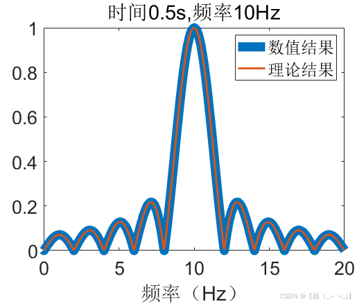
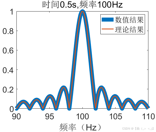
持续时间 的信号
的信号 的傅里叶变换为

当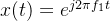 时,对应的频谱为:

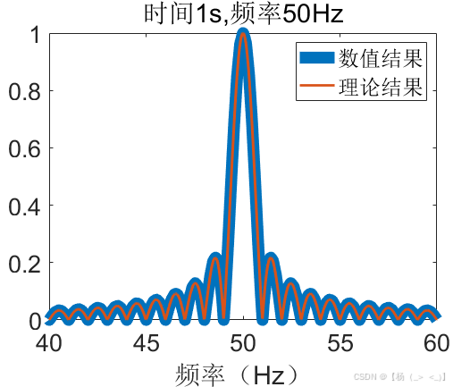
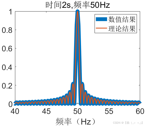
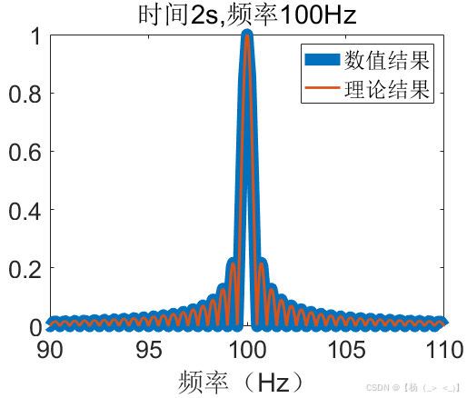
可以看出频率分辨率 与单频信号持续时间成反比,这意味着要想频率分辨性能好,单频信号持续时间要长。下面仿真不同持续时间、不同频率下的频谱结果。可以看出理论结果与数值结果高度吻合,且信号持续时间越长,频率分辨率越好。


1.2、时域分析和频域分析的优势和弊端
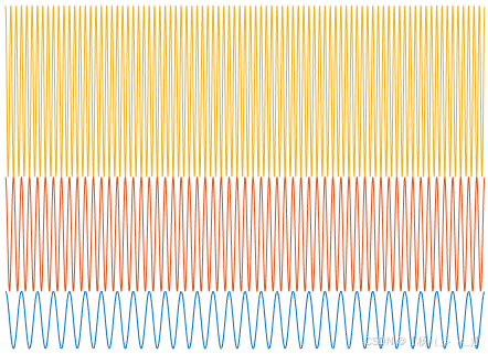
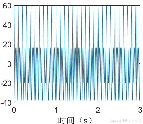
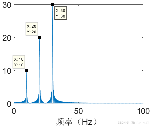
考虑信号持续时间内存在三个单频信号分量,幅度和频率分别为10,20,30下图分别表示各分量信号,混合信号,以及频谱。从中间的时域信号很难看出信号分量数量以及对应的参数值,而从频谱图上可以清晰的看出信号包含3个单频分量,并且可以准确估计三个分量的幅度和频率为10,20,30。从这里可以看出基于FFT的频域分析相比于时域分析的优势。
然而实际工程中存在的三个单频信号很大可能不会同时存在,可能会在不同的时间段内串行存在,考虑每个信号分量存在时间长度一样,则信号时域存在以下可能:
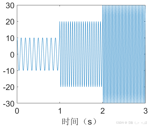


从时域可以清晰的看出,信号分量时域突变的时间点,即各分量信号的起始时间以及终止时间,下图展示了对应的频谱结果,可以看出频谱分析并不能得到信号分量的时域特征。


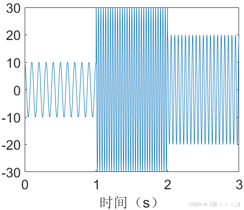
当信号分量存在时间有交叉时,信号时域、频域表示如下图所示,可以看出信号的起始时刻很难通过时域分析、频域分析得到,需要联合时域-频域特征才能得到,即时频分析。


结论:时域分析可以得到信号的时域特征,尤其是信号时域突变特征;频域分析可以得到信号的频率特征,尤其是信号分量的频率成分。当分量信号存在时频混叠时,联合时域分析和频域分析无法完全解析混合信号的时域特征以及频域特征。
二、线性时频分析
2.1、短时傅里叶变换(分辨率固定)

持续时间的信号的短时傅里叶变换为

离散化结果

当窗函数 为矩形窗时,短时傅里叶变换结果受窗长度,以及窗移动距离影响。
2.2、小波变换(多分辨率)

持续时间的信号的连续小波变换为

其中 表示缩放因子,
 表示时延因子,式中系列函数
 称为小波函数,它是由母函数
 经过不同的时间尺度伸缩和不同的时间平移得到的。下图展示了短时傅里叶变换和小波变换的时频图,可以很清楚的看出,小波变换频率越低,频率分辨率越好,并且相比于短时傅里叶变换,具有更好的时间分辨性能。
2.3、S变换(Stockwell变换,多分辨率)

持续时间的信号的S变换为

2.4、分数阶傅里叶变换
持续时间的信号的分数阶傅里叶变换为

其中 ,
, ,
, 表示阶次,
表示阶次, 表示分数阶傅里叶域,当阶次为1时,上式退化为傅里叶变换。
三、非线性时频分析
3.1、二次型时频分析
Wigner-Ville分布(WVD)
持续时间的信号的Wigner-Ville分布为

由于是二次型时频分布,当存在时频混叠情况时,其时频图存在交叉项。
平滑Wigner-Ville分布(SWVD)
利用平滑函数 对Wigner-Ville分布进行二维卷积处理得到平滑Wigner-Ville分布

平滑函数可为高斯核:

通过牺牲时频分辨率来抑制交叉项。
伪Wigner-Ville分布(PWVD)
持续时间的信号的伪Wigner-Ville分布为

其中 ,是对信号的加窗滞后。凸显细节
平滑伪Wigner-Ville分布(SPWVD)
持续时间的信号的伪Wigner-Ville分布为

其中 和
和 都是平滑窗。
Cohen类分布
持续时间的信号的Cohen类分布为

 为时间,
为时间, 为频率,
为频率, 为时移,
为时移, 为频移,为积分变量。
 为时频分布核函数。
Choi-Williams分布
当 ,Cohen类分布为 Choi-Williams分布:

注:Affine类时频分布是在Wigner-Ville分布的基础上增加核函数来进行仿射平滑,保持了原有Wigner-Ville分布的时移和伸缩移不变性。
3.2、非线性时频分析
经验模态分解(EMD)
EMD是一种非线性的时频分析方法,适用于非线 性、非平稳信号的处理,它可以依据信号内部的时间尺度特征自适应分解信号,其 基函数即为信号本身,是由数据驱动的信号分解,适用于突变信号的处理分析。具体步骤如下:
1)对原始信号全部极大、小值点分别采用三次样条插值进行连接,求出上、 下包络曲线 、
、 ;
;
2)求取上、下包络曲线均值 ;
;
3)计算原信号与包络均值 的差值,得到信号分量
 ;
;
4)判断分量 是否满足IMF必要条件(IMF必要条件:在IMF分量整体中,局部极值点与过零点个数应相等或相差至多为1,极 值点包括极大值点与极小值点;对于IMF分量任意点,由极大、小值点确定的上、下包络均值为零。),若满足则令
 ,记作IMF 的第一个分量,若不满足则将带入步骤1)中作为初始输入开始再一轮计算, 重复1)-3)的过程k次,直至(c)的输出分量
 满足IMF约束条件,则记IMF 第一分量为
 ;
;
5)将原信号与IMF分量 作差,记为
作差,记为 ,对
,对 进行步骤 1)-4)的过程,不断循环直到出现残余项
 为一单调函数或常数时,停止分解。
筛分出的第一个模态分量包含原始信号的最高频率成分,之后分解出的IMF分量频率依次递减。原始信号经由EMD过程得到的IMF分量和残余项可表示为:
变分模态分解(VMD)
VMD可以将信号分解为具有固定带宽和中心频率的有限固有振荡模态,并要求各模态信号的频谱能量为紧支撑,具体步骤如下:
1)设定原始信号可以被分解为K个模态(可以通过EMD获得),每个模态函数 都包含一 中心频率
 及它的有效带宽,对进行希尔伯特变换,得单边谱
![c{}'_{k}\\left ( t \\right )=\\left [ \\delta \\left ( t \\right ) +\\frac{j}{\\pi t}\\right ]\\ast c_{k}\\left ( t \\right )](2025-06-06h2gkpen0j1m.png)
2)将解析信号 频谱搬移到基带:

3)构建使所有模态带宽之和最小的约束模型:
![\\begin{matrix} \\underset{c_{k}\\left ( t \\right ),f_{k}}{\\text{min}}\\sum_{k=1}^{K}\\left \\| \\partial _{t} \\left [ \\left ( \\delta \\left ( t \\right ) +\\frac{j}{\\pi t}\\right )\\ast c_{k}\\left ( t \\right )\\right ]e^{-j2\\pi f_{k}t}\\right \\|_{2}^{2}\\\\ s.t.\\sum_{k=1}^{K}c_{k}\\left ( t \\right )=x\\left ( t \\right ) \\end{matrix}](2025-06-06a4qsijxwhi2.png)
4)构造拉格朗日展开式如下:
5)最优解通过交替方向乘子法计算得到,初始化 ,
, ,,
,, ,,
,, 第
第 次更新结果表示如下:
6)当满足以下条件,迭代停止
四、MATLAB时频分析函数
Time-Domain Processing
ifestar2 – Instantaneous frequency estimation using AR2 modelisation.
instfreq – Instantaneous frequency estimation.
loctime – Time localization characteristics.
Frequency-Domain Processing
fmt – Fast Mellin transform
ifmt – Inverse fast Mellin transform.
locfreq – Frequency localization characteristics.
sgrpdlay – Group delay estimation.
Linear Time-Frequency Processing
tfrgabor – Gabor representation.
tfrstft – Short time Fourier transform.
Bilinear Time-Frequency Processing in the Cohen's Class
tfrbj – Born-Jordan distribution.
tfrbud – Butterworth distribution.
tfrcw – Choi-Williams distribution.
tfrgrd – Generalized rectangular distribution.
tfrmh – Margenau-Hill distribution.
tfrmhs – Margenau-Hill-Spectrogram distribution.
tfrmmce – MMCE combination of spectrograms.
tfrpage – Page distribution.
tfrpmh – Pseudo Margenau-Hill distribution.
tfrppage – Pseudo Page distribution.
tfrpwv – Pseudo Wigner-Ville distribution.
tfrri – Rihaczek distribution.
tfrridb – Reduced interference distribution (Bessel window).
tfrridh – Reduced interference distribution (Hanning window).
tfrridn – Reduced interference distribution (binomial window).
tfrridt – Reduced interference distribution (triangular window).
tfrsp – Spectrogram.
tfrspwv – Smoothed Pseudo Wigner-Ville distribution.
tfrwv – Wigner-Ville distribution.
tfrzam – Zhao-Atlas-Marks distribution.
Bilinear Time-Frequency Processing in the Affine Class
tfrbert – Unitary Bertrand distribution.
tfrdfla – D-Flandrin distribution.
tfrscalo – Scalogram, for Morlet or Mexican hat wavelet.
tfrspaw – Smoothed Pseudo Affine Wigner distributions.
tfrunter – Unterberger distribution, active or passive form.
Reassigned Time-Frequency Processing
tfrrgab – Reassigned Gabor spectrogram.
tfrrmsc – Reassigned Morlet Scalogram time-frequency distribution.
tfrrpmh – Reassigned Pseudo Margenau-Hill distribution.
tfrrppag – Reassigned Pseudo Page distribution.
tfrrpwv – Reassigned Pseudo Wigner-Ville distribution.
tfrrsp – Reassigned Spectrogram.
tfrrspwv – Reassigned Smoothed Pseudo WV distribution.
Ambiguity Functions
ambifunb – Narrow band ambiguity function.
ambifuwb – Wide band ambiguity function.
Post-Processing or Help to the Interpretation
friedman – Instantaneous frequency density.
holder – Estimate the Holder exponent through an affine TFR.
htl – Hough transform for detection of lines in images.
margtfr – Marginals and energy of a time-frequency representation.
midscomp – Mid-point construction used in the interference diagram.
momftfr – Frequency moments of a time-frequency representation.
momttfr – Time moments of a time-frequency representation.
plotsid – Schematic interference diagram of FM signals.
renyi – Measure Renyi information.
ridges – Extraction of ridges.
tfrideal – Ideal TFR for given frequency laws.
Visualization & backup
plotifl – Plot normalized instantaneous frequency laws.
tfrqview – Quick visualization of time-frequency representations.
tfrview – Visualization of time-frequency representations.
tfrparam – Return the paramaters needed to display (or save) a TFR.
tfrsave – Save the parameters of a time-frequency representation.
Other
disprog – Display progression of a loop.
divider – Find dividers of integer such that product equals integer.
dwindow – Derive a window.
integ – Approximate integral.
integ2d – Approximate 2-D integral.
izak – Inverse Zak transform.
istfr1 – returns true if a distribution is Cohen's class type 1 (spectrogram)
istfr2 – returns true if a distribution is Cohen's class type 2 (Wigner-Ville)
istfraff – returns true is a distribution is an affine class member
kaytth – Kay-Tretter filter computation.
modulo – Congruence of a vector.
movcw4at – Four atoms rotating, analyzed by the Choi-Williams distribution.
movpwdph – Influence of a phase-shift on the interferences of the pWVD.
movpwjph – Influence of a jump of phase on the interferences of the pWVD.
movsc2wv – Movie illustrating the passage from the scalogram to the WVD.
movsp2wv – Movie illustrating the passage from the spectrogram to the WVD.
movwv2at – Oscillating structure of the interferences of the WVD.
odd – Round towards nearest odd value.
sigmerge – Add two signals with given energy ratio in dB.
zak – Zak transform.
部分文献
[1] Y. Chen and K. Sun, "A BeiDou Sweep Interference Detection Method based on Choi-Williams-Hough transform," 2022 7th International Conference on Intelligent Computing and Signal Processing (ICSP), Xi'an, China, 2022, pp. 589-593
[2] Variational Mode Decomposition (变分模态分解)
[3] 邵丹.地震数据时频特征优化与基于学习模型的消噪算法研究[D].吉林大学,2024.
总结
本文较为详细的分析傅里叶变换方法的优势以及局限性,并总结各类时频分析方法。后续将结合仿真具体展开分析。转载请附上链接:【杨(_> <_)】的博客_CSDN博客-信号处理,SAR,代码实现领域博主


评论前必须登录!
注册