一篇文章搞清楚数据库(下)

单表约束_介绍

约束介绍:
概述:
约束可以理解为在数据类型的基础上, 继续都某列数据值 做限定, 例如: 不能重复, 不能为空等…
专业版: 约束是用来保证数据的完整性 和 安全性的.
分类:
单表约束:
主键约束: primary key
特点: 非空, 唯一, 一般结合 auto_increment(自动增长) 一起使用.
非空约束: not null
特点: 该列值不能为空, 但是可以: 重复.
唯一约束: unique
特点: 该列值不能重复, 但是可以: 为空.
默认约束: default 默认值
特点: 如果添加数据的时候没有给值, 就用默认值填充. 类似于Python中的 缺省参数(默认参数)
多表约束:
主外键约束: foreign key

# ——————— 单表约束 ———————
/*
约束介绍:
概述:
约束可以理解为在数据类型的基础上, 继续都某列数据值 做限定, 例如: 不能重复, 不能为空等…
专业版: 约束是用来保证数据的完整性 和 安全性的.
分类:
单表约束:
主键约束: primary key
特点: 非空, 唯一, 一般结合 auto_increment(自动增长) 一起使用.
非空约束: not null
特点: 该列值不能为空, 但是可以: 重复.
唯一约束: unique
特点: 该列值不能重复, 但是可以: 为空.
默认约束: default 默认值
特点: 如果添加数据的时候没有给值, 就用默认值填充. 类似于Python中的 缺省参数(默认参数)
多表约束:
主外键约束: foreign key
*/
— 1. 创建数据库.
drop database tb;
create database tb charset 'utf8';
— 2. 切库.
use tb;
— 3. 查看数据表.
show tables;
— 4. 创建数据表, 用于演示单表约束.
create table if not exists stu(
id int primary key auto_increment, # id列, 主键列(非空,唯一), 自增
name varchar(10) not null, # 姓名, 不能为空
phone varchar(11) unique, # 手机号, 唯一
gender varchar(2), # 性别, 没有限定.
address varchar(10) default '北京' # 默认约束
);
# 5. 往表中添加数据, 用于测试: 约束.
# 正常添加结果
insert into stu values(null, '杨过', '111', '男', '上海');
insert into stu values(null, '郭靖', '222', '男', '广州');
insert into stu values(null, '黄蓉', '333', '女', '深圳');
# 测试 默认约束
insert into stu(id, name, phone, gender) values(null, '尹志平', '444', '男');
# 测试 非空约束.
insert into stu values(null, null, '555', '女', '深圳'); # 报错, Column 'name' cannot be null
# 测试 唯一约束
insert into stu values(null, '黄蓉', '555', '女', '深圳');
insert into stu values(null, '黄蓉', null, '女', '深圳');
insert into stu values(null, '黄蓉', '555', '女', '深圳'); # 报错, Duplicate entry '555' for key 'phone'
# 6. 查看表数据.
select * from stu;
# 7. 查看表结构
desc stu;

单表查询_简单查询

单表查询, 完整查询格式如下:
select
[distinct] 列名1 as 别名, 列名2 as 别名, …
from
数据表名
where
组前筛选
group by
分组字段
having
组后筛选
order by
排序字段 [asc | desc]
limit
起始索引, 数据条数;

# ——————— 单表查询 -> 简单查询 ———————
/*
单表查询, 完整查询格式如下:
select
[distinct] 列名1 as 别名, 列名2 as 别名, …
from
数据表名
where
组前筛选
group by
分组字段
having
组后筛选
order by
排序字段 [asc | desc]
limit
起始索引, 数据条数;
*/
# 1. 创建商品表.
create table product
(
pid int primary key auto_increment, # 商品id, 主键
pname varchar(20), # 商品名
price double, # 商品单价
category_id varchar(32) # 商品的分类id
);

# 2. 添加表数据.
INSERT INTO product(pid,pname,price,category_id) VALUES(null,'联想',5000,'c001');
INSERT INTO product(pid,pname,price,category_id) VALUES(null,'海尔',3000,'c001');
INSERT INTO product(pid,pname,price,category_id) VALUES(null,'雷神',5000,'c001');
INSERT INTO product(pid,pname,price,category_id) VALUES(null,'杰克琼斯',800,'c002');
INSERT INTO product(pid,pname,price,category_id) VALUES(null,'真维斯',200, null);
INSERT INTO product(pid,pname,price,category_id) VALUES(null,'花花公子',440,'c002');
INSERT INTO product(pid,pname,price,category_id) VALUES(null,'劲霸',2000,'c002');
INSERT INTO product(pid,pname,price,category_id) VALUES(null,'香奈儿',800,'c003');
INSERT INTO product(pid,pname,price,category_id) VALUES(null,'相宜本草',200, null);
INSERT INTO product(pid,pname,price,category_id) VALUES(null,'面霸',5,'c003');
INSERT INTO product(pid,pname,price,category_id) VALUES(null,'好想你枣',56,'c004');
INSERT INTO product(pid,pname,price,category_id) VALUES(null,'香飘飘奶茶',1,'c005');
INSERT INTO product(pid,pname,price,category_id) VALUES(null,'海澜之家',1,'c002');

# 3. 查看表数据.
# 需求1: 查询所有的商品信息
select * from product;
select pid, pname, price, category_id from product; # 效果同上.

# 需求2: 查看商品名 和 商品价格.
select pname, price from product;
# 扩展: 起别名, 列名, 表名都可以起别名.
# 格式: 列名 as 别名 或者 表名 as 别名, 其中 as 可以省略不写.
select pname as 商品名, price 商品价格 from product as p;

# 需求3: 查看结果是表达式, 将所有的商品价格+10, 进行展示.
select pname, price + 10 from product;
select pname, price + 10 as price from product;

条件查询_比较运算符

# ——————— 单表查询 -> 条件查询 ———————
# 格式: select 列名1, 列名2… from 数据表名 where 条件;
# 场景1: 比较运算符, >, >=, <, <=, =, !=, <>
# 需求1: 查询商品名称为“花花公子”的商品所有信息：
select * from product where pname ='花花公子';
# 需求2: 查询价格为800商品
select * from product where price=800;
# 需求3: 查询价格不是800的所有商品
select * from product where price!=800;
select * from product where price<>800;
# 需求4: 查询商品价格大于60元的所有商品信息
select * from product where price > 60;
# 需求5: 查询商品价格小于等于800元的所有商品信息
select * from product where price <= 800;

条件查询_逻辑运算符和范围查询

# 场景2: 范围查询. between 值1 and 值2 -> 适用于连续的区间, in (值1, 值2..) -> 适用于 固定值的判断.
# 场景3: 逻辑运算符. and, or, not
# 需求6: 查询商品价格在200到800之间所有商品
select * from product where price between 200 and 800; # 包左包右.
select * from product where price >= 200 and price <= 800;

# 需求7: 查询商品价格是200或800的所有商品
select * from product where price in (200, 800);
select * from product where price=200 or price=800;

# 需求8: 查询价格不是800的所有商品
select * from product where price != 800;
select * from product where not price = 800;
select * from product where price not in (800);

条件判断_模糊查询和非空判断

# 场景4: 模糊查询. 字段名 like '_内容%' _ 代表任意的1个字符; %代表任意的多个字符, 至少0个, 至多无所谓.
# 需求9: 查询以'香'开头的所有商品
select * from product where pname like '香%';
# 需求10: 查询第二个字为'想'的所有商品
select * from product where pname like '_想%';
select * from product where pname like '_想'; # 只能查出 *想 两个字的, 不符合题设.

# 场景5: 非空查询. is null, is not null, 不能用=来判断空.
# 需求11: 查询没有分类的商品
select * from product where category_id=null; # 不报错,但是没结果.
select * from product where category_id is null; # 正确的, 判空操作.

# 需求12: 查询有分类的商品
select * from product where category_id is not null; # 正确的, 非空判断操作.

排序查询

# ——————— 单表查询 -> 排序查询 ———————
# 格式: select * from 表名 order by 排序的字段1 [asc | desc], 排序的字段2 [asc | desc], …;
# 解释1: ascending: 升序, descending: 降序.
# 解释2: 默认是升序, 所以asc可以省略不写.
# 需求1: 根据价格降序排列.
select * from product order by price; # 默认是: 升序.
select * from product order by price asc; # 效果同上.
select * from product order by price desc; # 价格降序排列.

# 需求2: 根据价格降序排列, 价格一样的情况下, 根据分类降序排列.
select * from product order by price desc, category_id desc;

聚合查询

聚合查询(多进一出)介绍:
概述:
聚合查询是对表中的某列数据做操作.
常用的聚合函数:
count() 统计某列值的个数, 只统计非空值. 一般用于统计 表中数据的总条数.
sum() 求和
max() 求最大值
min() 求最小值
avg() 求平均值
面试题: count(), count(1), count(列)的区别是什么?
区别1: 是否统计空值
count(列): 只统计该列的非空值.
count(1), count(): 统计所有数据, 包括空值.
区别2: 效率问题.
1. COUNT() 和 COUNT(1) —— 最快
InnoDB 会直接读取聚簇索引（PRIMARY KEY）的行数计数器（近似 O(1)），无需扫描数据页。
优化器将两者视为等价，生成相同执行计划。
✅ 推荐用于统计总行数。
2. COUNT(主键列) —— 次快
主键列是聚簇索引的一部分，InnoDB 可通过遍历主键索引（B+树叶子节点）计数。
虽然仍需扫描索引页，但避免回表，比全表扫描快。
⚠️ 若主键是联合主键或非整型，性能略低于 COUNT()。
3. COUNT(普通列) —— 最慢
若该列无索引：需全表扫描（type: ALL），逐行判断是否为 NULL。
若该列有二级索引：可能走索引扫描（type: index），但仍需访问索引页并过滤 NULL。
❗ 当列含大量 NULL 时，优化器无法使用元数据，必须实际计算。

# ——————— 单表查询 -> 聚合查询 ———————
/*
聚合查询(多进一出)介绍:
概述:
聚合查询是对表中的某列数据做操作.
常用的聚合函数:
count() 统计某列值的个数, 只统计非空值. 一般用于统计 表中数据的总条数.
sum() 求和
max() 求最大值
min() 求最小值
avg() 求平均值
面试题: count(*), count(1), count(列)的区别是什么?
区别1: 是否统计空值
count(列): 只统计该列的非空值.
count(1), count(*): 统计所有数据, 包括空值.
区别2: 效率问题.
1. COUNT(*) 和 COUNT(1) —— 最快
InnoDB 会直接读取聚簇索引（PRIMARY KEY）的行数计数器（近似 O(1)），无需扫描数据页。
优化器将两者视为等价，生成相同执行计划。
✅ 推荐用于统计总行数。
2. COUNT(主键列) —— 次快
主键列是聚簇索引的一部分，InnoDB 可通过遍历主键索引（B+树叶子节点）计数。
虽然仍需扫描索引页，但避免回表，比全表扫描快。
⚠️ 若主键是联合主键或非整型，性能略低于 COUNT(*)。
3. COUNT(普通列) —— 最慢
若该列无索引：需全表扫描（type: ALL），逐行判断是否为 NULL。
若该列有二级索引：可能走索引扫描（type: index），但仍需访问索引页并过滤 NULL。
❗ 当列含大量 NULL 时，优化器无法使用元数据，必须实际计算。
*/
# 需求1: 查询商品的总条数
select count(pid) as total_cnt from product;
select count(category_id) as total_cnt from product;
select count(*) as total_cnt from product;
select count(1) as total_cnt from product;

# 需求2: 查询价格大于200商品的总条数
select count(pid) as total_cnt from product where price > 200;

# 需求3: 查询分类为'c001'的所有商品价格的总和
select sum(price) as total_price from product where category_id='c001';

# 需求4: 查询分类为'c002'所有商品的平均价格
select avg(price) as avg_price from product where category_id='c002';

# 需求5: 查询商品的最大价格和最小价格 扩展: ctrl + alt + 字母L 代码格式化.
select
max(price) as max_price,
min(price) as min_price
from
product;

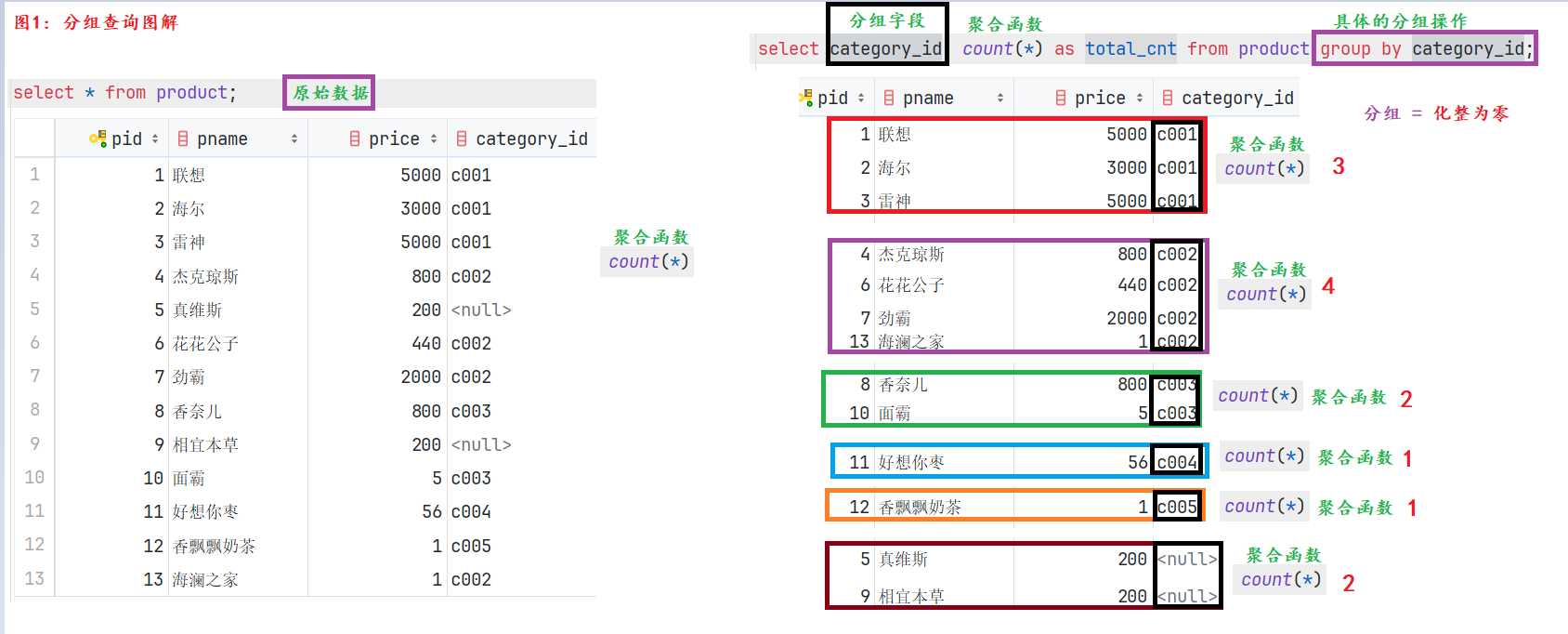
分组查询

分组查询介绍:
概述:
简单理解为, 根据分组字段, 把表数据 化整为零, 然后基于每个分组后的每个部分, 进行对应的聚合运算.
格式:
select 列1, 列2… from 数据表名 where 组前筛选 group by 分组字段 having 组后筛选;
细节:
1. 分组查询 一般要结合 聚合函数一起使用, 且根据谁分组, 就根据谁查询.
2. 组前筛选用where, 组后筛选用having.
3. 面试题: where 和 having的区别是什么?
where: 组前筛选, 后边不能跟聚合函数.
having: 组后筛选, 后边可以跟聚合函数.
4. 分组查询的查询列 只能出现 分组字段, 聚合函数.
5. 如果只分组, 没有写聚合, 可以理解为是: 基于分组字段, 进行去重查询

# ——————— 单表查询 -> 分组查询 ———————
/*
分组查询介绍:
概述:
简单理解为, 根据分组字段, 把表数据 化整为零, 然后基于每个分组后的每个部分, 进行对应的聚合运算.
格式:
select 列1, 列2… from 数据表名 where 组前筛选 group by 分组字段 having 组后筛选;
细节:
1. 分组查询 一般要结合 聚合函数一起使用, 且根据谁分组, 就根据谁查询.
2. 组前筛选用where, 组后筛选用having.
3. 面试题: where 和 having的区别是什么?
where: 组前筛选, 后边不能跟聚合函数.
having: 组后筛选, 后边可以跟聚合函数.
4. 分组查询的查询列 只能出现 分组字段, 聚合函数.
5. 如果只分组, 没有写聚合, 可以理解为是: 基于分组字段, 进行去重查询
*/
# 需求1: 统计各个分类商品的个数.
select category_id, count(*) as total_cnt from product group by category_id;

# 需求2: 统计各个分类商品的个数, 且只显示个数大于1的信息.
select
category_id,
count(*) as total_cnt
from
product
group by
category_id # 根据商品类别分组.
having
total_cnt > 1; # 组后筛选

# 需求3: 演示 如果只分组, 没有写聚合, 可以理解为是: 基于分组字段, 进行去重查询
select category_id from product group by category_id;
select category_id from product group by category_id;

# 还可以通过 distinct 关键字来实现去重.
select distinct category_id from product;

# 此时是: 按照category_id 和 price作为整体, 然后去重.
select distinct category_id, price from product;
select category_id, price from product group by category_id, price; # 效果同上.

分页查询

分页查询介绍:
概述:
分页查询 = 每次从数据表中查询出固定条数的数据, 一方面可以降低服务器的压力, 另一方面可以降低浏览器端的压力, 且可以提高用户体验.
实际开发中非常常用.
格式:
limit 起始索引, 数据条数;
细节:
1. 表中每条数据都有自己的索引, 且索引是从0开始的.
2. 如果是从索引0开始获取数据的, 则索引0可以省略不写.
学好分页, 掌握如下的几个参数计算规则即可:
数据总条数: count() 函数
每页的数据条数: 产品说了算
每页的起始索引: (当前的页数 – 1) * 每页的数据条数
总页数: (数据总条数 + 每页的数据条数 – 1) // 每页的数据条数
(13 + 5 – 1) // 5 = 17 // 5 = 3页
(14 + 5 – 1) // 5 = 18 // 5 = 3页
(15 + 5 – 1) // 5 = 19 // 5 = 3页
(16 + 5 – 1) // 5 = 20 // 5 = 4页

# ——————— 单表查询 -> 分页查询 ———————
/*
分页查询介绍:
概述:
分页查询 = 每次从数据表中查询出固定条数的数据, 一方面可以降低服务器的压力, 另一方面可以降低浏览器端的压力, 且可以提高用户体验.
实际开发中非常常用.
格式:
limit 起始索引, 数据条数;
细节:
1. 表中每条数据都有自己的索引, 且索引是从0开始的.
2. 如果是从索引0开始获取数据的, 则索引0可以省略不写.
学好分页, 掌握如下的几个参数计算规则即可:
数据总条数: count() 函数
每页的数据条数: 产品说了算
每页的起始索引: (当前的页数 – 1) * 每页的数据条数
总页数: (数据总条数 + 每页的数据条数 – 1) // 每页的数据条数
(13 + 5 – 1) // 5 = 17 // 5 = 3页
(14 + 5 – 1) // 5 = 18 // 5 = 3页
(15 + 5 – 1) // 5 = 19 // 5 = 3页
(16 + 5 – 1) // 5 = 20 // 5 = 4页
*/
# 需求1: 5条/页.
select * from product limit 5; # 第1页, 从索引0开始, 获取5条.
select * from product limit 0, 5; # 第1页, 从索引0开始, 获取5条, 效果同上.

select * from product limit 0, 5; # 第1页, 从索引0开始, 获取5条.
select * from product limit 5, 5; # 第2页, 从索引5开始, 获取5条.

# 需求2: 3条/页
select * from product limit 0, 3; # 第1页, 从索引0开始, 获取3条.
select * from product limit 3, 3; # 第2页, 从索引3开始, 获取3条.
select * from product limit 6, 3; # 第3页, 从索引6开始, 获取3条.
select * from product limit 9, 3; # 第4页, 从索引9开始, 获取3条.
select * from product limit 12, 3; # 第5页, 从索引12开始, 获取3条.

# 总结, 回顾单表查询的格式
/*
select
[distinct] 列1 as 别名, 列2
from
数据表名
where
组前筛选
group by
分组字段
having
组后筛选
order by
排序字段 [asc | desc]
limit
起始索引, 数据条数;
*/
# 需求: 统计商品表中, 每类商品的单价总和, 只统计单价在100以上的商品, 只查看单价总和在500以上的分类, 按照商品总价降序排列, 只获取商品总价高的前2条数信息.
select
category_id,
sum(price) total_price
from
product
where # 组前筛选
price > 100
group by # 分组
category_id
having # 组后筛选
total_price > 500
order by # 排序
total_price desc
limit 0, 2; # 分页

多表建表_一对多

• 图解

  

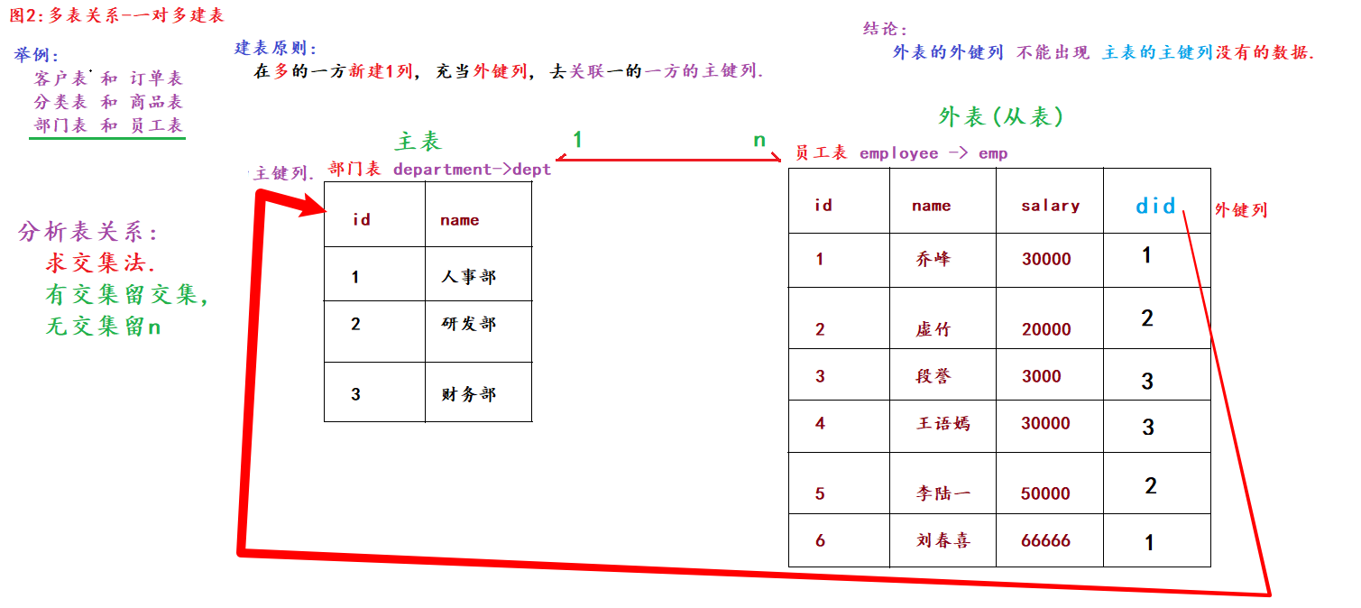
多表关系解释:
概述:
MySQL是一种关系型数据库, 采用 数据表 来存储数据, 且表与表之间是有关系的.
例如: 一对多, 多对多, 一对一…
举例:
一对多: 部门表和员工表, 客户表和订单表, 分类表和商品表…
多对多: 学生表和选修课表, 订单表和商品表, 学生表和老师表…
一对一: 一个人有1个身份证号, 1家公司只有1个注册地址, 1个法人.
建表原则:
一对多: 在多的一方新建1列, 充当外键列, 去关联1的一方的主键列.
多对多: 新建中间表. 该表至少有3列(自身主键, 剩下两个当外键), 分别去关联多的两方的主键列.
一对一: 直接放到一张表中.
结论(记忆):
1. 外表的外键列, 不能出现主表的主键列没有的数据.
2. 约束是用来保证数据的完整性和安全性的.
3. 添加 和 删除外键约束的格式如下:
添加外键约束: alter table 外表名 add [constraint 外键约束名] foreign key(外键列名) references 主表名(主键列名);
删除外键约束: alter table 外表名 drop foreign key 外键约束名;

• 代码

  # ———————- 多表建表 一对多关系 ———————-
  /*
  多表关系解释:
  概述:
  MySQL是一种关系型数据库, 采用 数据表 来存储数据, 且表与表之间是有关系的.
  例如: 一对多, 多对多, 一对一…
  举例:
  一对多: 部门表和员工表, 客户表和订单表, 分类表和商品表…
  多对多: 学生表和选修课表, 订单表和商品表, 学生表和老师表…
  一对一: 一个人有1个身份证号, 1家公司只有1个注册地址, 1个法人.
  建表原则:
  一对多: 在多的一方新建1列, 充当外键列, 去关联1的一方的主键列.
  多对多: 新建中间表. 该表至少有3列(自身主键, 剩下两个当外键), 分别去关联多的两方的主键列.
  一对一: 直接放到一张表中.
  结论(记忆):
  1. 外表的外键列, 不能出现主表的主键列没有的数据.
  2. 约束是用来保证数据的完整性和安全性的.
  3. 添加 和 删除外键约束的格式如下:
  添加外键约束: alter table 外表名 add [constraint 外键约束名] foreign key(外键列名) references 主表名(主键列名);
  删除外键约束: alter table 外表名 drop foreign key 外键约束名;
  */
  # 1. 切库, 查表.
  use tb;
  show tables;

  # 2. 新建部门表.
  drop table dept;
  create table dept(
  id int primary key auto_increment, # 部门id
  name varchar(10) # 部门名字
  );

  # 3. 新建员工表, 指定外键列.
  drop table emp;
  create table emp(
  id int primary key auto_increment, # 员工id
  name varchar(10), # 员工姓名
  salary int, # 员工工资
  dept_id int # 员工所属的部门id
  # 方式1: 建表时, 直接添加外键.
  # , constraint fk_dept_emp foreign key(dept_id) references dept(id)
  , foreign key(dept_id) references dept(id)
  );

  # 方式2: 建表后, 添加外键.
  alter table emp add constraint fk_01 foreign key(dept_id) references dept(id);

  # 4. 添加数据.
  insert into dept values(null, '人事部'), (null, '研发部'), (null, '财务部');
  insert into emp values
  (null, '乔峰', 30000, 1),
  (null, '虚竹', 20000, 2),
  (null, '段誉', 3000, 3);
  # 尝试添加脏数据.
  insert into emp values(null, '喜哥', 66666, 10);
  # 5. 查看表数据.
  select * from dept;
  select * from emp;
  # 6. 删除外键约束.
  alter table emp drop foreign key emp_ibfk_1;

多表查询_交叉查询

# ———————- 多表查询 准备数据 ———————-
# 1. 创建hero表
create table hero (
hid int primary key auto_increment, # 英雄id
hname varchar(255), # 英雄名
kongfu_id int # 功夫id
);
# 2. 创建kongfu表
create table kongfu (
kid int primary key auto_increment, # 功夫id
kname varchar(255) # 功夫名
);
# 3. 添加表数据.
# 插入hero数据
insert into hero values(1, '鸠摩智', 9),(3, '乔峰', 1),(4, '虚竹', 4),(5, '段誉', 12);
# 插入kongfu数据
insert into kongfu values(1, '降龙十八掌'),(2, '乾坤大挪移'),(3, '猴子偷桃'),(4, '天山折梅手');
# 4. 查看表数据.
select * from hero;
select * from kongfu;

# 多表查询的精髓是: 根据 关联条件 和 组合方式, 把多张表组成1张表, 然后进行 单表查询.
# ———————- 多表查询 交叉查询 ———————-
# 格式: select * from 表A, 表B;
# 结果: 表A的总条数 * 表B的总条数 -> 笛卡尔积, 一般不用.
select * from hero, kongfu;

多表查询_内连接

# ———————- 多表查询 连接查询 ———————-
# 场景1: 内连接, 查询结果 = 表的交集.
# 格式1: select * from 表A inner join 表B on 关联条件; 显式内连接(推荐)
select * from hero h inner join kongfu kf on h.kongfu_id = kf.kid;
select * from hero h join kongfu kf on h.kongfu_id = kf.kid; # inner可以省略不写.
select * from hero h join kongfu kf on kongfu_id = kid; # 如果两张表没有重名字段, 则: 可以省略 表名. 的方式.

# 格式2: select * from 表A, 表B where 关联条件; 隐式内连接,性能堪忧
select * from hero h, kongfu kf where h.kongfu_id = kf.kid;

多表查询_外连接

# 场景2: 外连接
# 格式1: 左外连接, 查询结果 = 左表的全集 + 表的交集.
# 格式: select * from 表A left outer join 表B on 关联条件;
select * from hero h left outer join kongfu kf on h.kongfu_id = kf.kid;
select * from hero left join kongfu on kongfu_id = kid; # 简化版写法.

# 格式2: 右外连接, 查询结果 = 右表的全集 + 表的交集.
# 格式: select * from 表A right outer join 表B on 关联条件;
select * from hero h right outer join kongfu kf on h.kongfu_id = kf.kid;
select * from hero right join kongfu on kongfu_id = kid; # 简化版写法.

# 结论: 如果交换了表的顺序, 则左外连接和右外连接, 查询结果可以是一样的. 掌握一种即可, 推荐: 左外连接.
# 左外连接.
select * from kongfu left join hero on kongfu_id = kid;
# 右外连接.
select * from hero right join kongfu on kongfu_id = kid;

多表查询_子查询

# ———————- 多表查询 子查询(套娃写法,不推荐,性能堪忧,可以选择用联表查来代替) ———————-
/*
概述:
如果1个查询语句的 查询条件 需要依赖另一个SQL语句的查询结果, 这种写法就称之为: 子查询.
叫法:
里边的查询叫: 子查询.
外边的查询叫: 父查询(主查询)
*/
# 1. 查看商品表的数据信息.
select * from product;

# 2. 需求: 查询商品表中所有单价在 均价之上的商品信息.
# 扩展: 四舍五入, 保留3位小数.
select round(1346.3846153846155, 3);

# 思路1: 分解版.
# step1: 查询所有商品的均价.
select round(avg(price), 3) avg_price from product;

# step2: 查询商品表中所有单价在 均价之上的商品信息.
select * from product where price > 1346.385;

# 思路2: 子查询.(套娃)
# 主查询(父查询) 子查询
select * from product where price > (select round(avg(price), 3) avg_price from product);

#思路3: 性能版(推荐)
select * from product
join (select round(avg(price),3) avg_price from product) avg_tb
on price > avg_price;

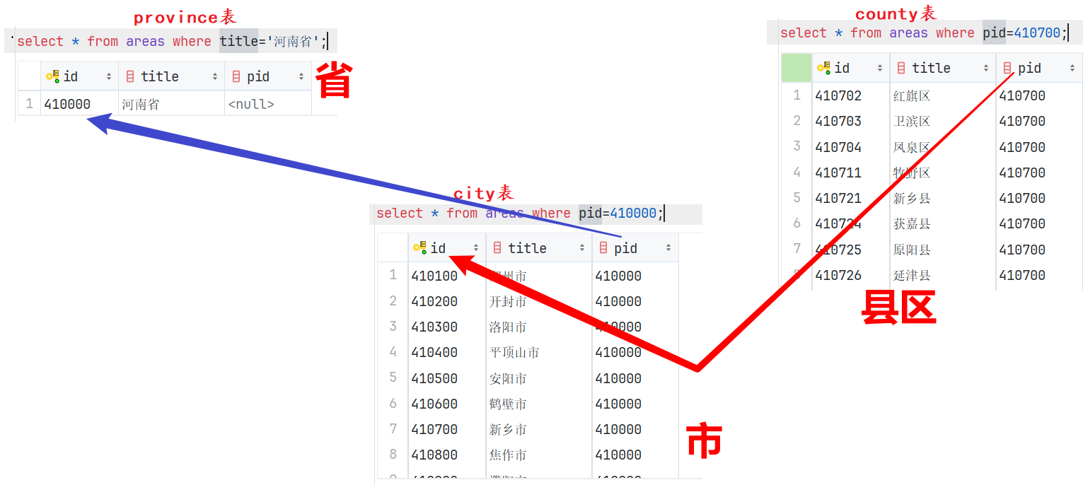
多表查询_自关联查询

• 图解

  

• 代码

  # ———————-多表查询 自关联查询 ———————-
  /*
  解释:
  表自己和自己做关联查询, 称之为: 自关联(自连接)查询.
  写法:
  可以是交叉查询, 内连接, 外连接…
  经典案例:
  行政区域表 -> 省市区.

  例如: 记录省市区的信息,
  复杂的写法: 搞三张表, 分别记录省, 市, 区的关系.
  简单的写法: 用1张表存储, 然后用的时候, 通过 自关联查询 实现即可.
  字段: 自身id 自身名字 父级id
  410000 河南省 0

  410100 郑州市 410000
  410200 开封市 410000
  410300 洛阳市 410000
  410700 新乡市 410000

  410101 二七区 410100
  410102 经开区 410100
  410701 红旗区 410700
  410702 卫滨区 410700
  410721 新乡县 410700
  */
  # 1. 查看区域表的信息.
  select * from areas;

  # 2. 查询河南省的信息.
  select * from areas where title='河南省';

  # 3. 查看河南省所有的市.
  select * from areas where pid=410000;

  # 4. 查看新乡市所有的县区.
  select * from areas where pid=410700;

  # 5. 查看河南省所有的市, 县区信息.
  select
  province.id, province.title, # 省的id, 名字
  city.id, city.title, # 市的id, 名字
  county.id, county.title # 县区的id, 名字
  from
  areas as county # 县区
  join
  areas as city on county.pid = city.id # 市
  join
  areas as province on city.pid = province.id # 省
  where
  province.title='河南省';

  # 6. 根据你的身份证号前6位, 查询你的家乡.
  select
  province.id, province.title, # 省的id, 名字
  city.id, city.title, # 市的id, 名字
  county.id, county.title # 县区的id, 名字
  from
  areas as county # 县区
  join
  areas as city on county.pid = city.id # 市
  join
  areas as province on city.pid = province.id # 省
  where
  county.id='320321';

  case when写法

格式1: 通用写法.
case
when 条件1 then 结果1
when 条件2 then 结果2
…
else 结果n
end [as 别名]
格式2: 针对于格式1的语法糖, 要满足两点 -> 1.都是操作同1个字段. 2.都是等于的判断.
case 字段名
when 值1 then 结果1
when 值2 then 结果2
…
else 结果n
end [as 别名]

select * from product;

/*
格式1: 通用写法.
case
when 条件1 then 结果1
when 条件2 then 结果2
…
else 结果n
end [as 别名]

格式2: 针对于格式1的语法糖, 要满足两点 -> 1.都是操作同1个字段. 2.都是等于的判断.
case 字段名
when 值1 then 结果1
when 值2 then 结果2
…
else 结果n
end [as 别名]
*/
# 需求: c001 -> 电脑, c002 -> 服装, c003 -> 化妆品, c004 -> 零食, c005 -> 饮料, null -> 未知类别
select
*,
case
when category_id = 'c001' then '电脑'
when category_id = 'c002' then '服装'
when category_id = 'c003' then '化妆品'
when category_id = 'c004' then '零食'
when category_id = 'c005' then '饮料'
else '未知类别'
end as category_name
from
product;

# 上述格式可以简化为
select
*,
case category_id
when 'c001' then '电脑'
when 'c002' then '服装'
when 'c003' then '化妆品'
when 'c004' then '零食'
when 'c005' then '饮料'
else '未知类别'
end as category_name
from
product;

if判断

select if(2 > 1, 2, 1); # if函数: if(条件,2,1),成立返回2,不成立返回1,等价于python中的三元表达式

# 需求:统计所有的订单,将价格分为高中低三档,报表输出三个字段统计数量情况
select
count(if(price<=500,1,null)) as 低,
count(if(price>500 and price<=2000,1,null)) as 中,
count(if(price>2000,1,null)) as 高
from product;

# 当然上述需求还可以这样完成
select case
when price > 2000 then '高'
when price <= 500 then '低'
else '中'
end as price_leavel,
count(1) as count
from product
group by price_leavel;

/*
以下是我问的ai的两种解法的对比情况,朋友们自行选择
方案一：单行聚合（COUNT(IF(…))）
特点：
结果格式：单行三列（低, 中, 高），适合报表直接展示。
逻辑：
IF(condition, 1, NULL)：满足条件返回 1，否则 NULL
COUNT(expr) 仅统计非 NULL 值 → 实现条件计数
性能：
仅一次全表扫描（type: ALL）
无排序、无分组，开销最小
若需求明确为“输出三列统计数”，用方案一

方案二：分组聚合（CASE + GROUP BY）
特点：
结果格式：多行两列（每档一行），适合后续程序处理或动态渲染。
逻辑：
CASE 动态生成分档标签
GROUP BY price_leavel 按标签分组计数
性能：
一次全表扫描 + 内部哈希分组（InnoDB 中 GROUP BY 可能使用临时表或 filesort）
比方案一略慢（尤其数据量大时）
优势：
语义更清晰，易于扩展（如加新档位、排序）
自动处理边界：price = 500 或 2000 归入 中（因 ELSE 覆盖）
若需灵活扩展或对接后端 API，用方案二（更符合 SQL 标准实践）
*/

窗口函数(M有SQL8.X 新特性)

窗口函数解释:
概述:
它是MySQL8.x的新特性, 主要用于 给表新增1列, 至于新增的内容是什么, 取决于你用什么 窗口函数.
格式:
窗口函数 over([partition by 分组字段 order by 排序字段 asc | desc])
常用的窗口函数:
row_number(): 做行号标记的, 即: 1, 2, 3, 4…
rank(): 做稀疏排名的.
dense_rank(): 做密集排名的.
大白话解释:
假设数据集是 100, 90, 90, 60, 则三个函数的排名结果分别是:
row_number(): 1, 2, 3, 4
rank(): 1, 2, 2, 4
dense_rank(): 1, 2, 2, 3
细节:
1. 窗口函数 = 给表新增1列, 至于新增的是什么, 取决于和什么函数一起用.
2. 如果不写partition by, 则统计的是全表数据, 如果写了, 则统计的是组内的数据.
3. 如果不写order by, 则统计的是组内所有的数据, 如果写了, 则统计的是组内从第一行, 截止到当前行的数据.
4. 可以尝试玩下其它的窗口函数结合over()一起用,
例如: count(), max(), min(), sum(), avg(), ntile(n), lag(), lead(), first_value(), last_value()…
总结: 关于窗口函数, 至少掌握两点:
1. 分组排名.
2. 分组排名求TopN

# ———————- 窗口函数(M有SQL8.X 新特性) ———————-
/*
窗口函数解释:
概述:
它是MySQL8.x的新特性, 主要用于 给表新增1列, 至于新增的内容是什么, 取决于你用什么 窗口函数.
格式:
窗口函数 over([partition by 分组字段 order by 排序字段 asc | desc])
常用的窗口函数:
row_number(): 做行号标记的, 即: 1, 2, 3, 4…
rank(): 做稀疏排名的.
dense_rank(): 做密集排名的.
大白话解释:
假设数据集是 100, 90, 90, 60, 则三个函数的排名结果分别是:
row_number(): 1, 2, 3, 4
rank(): 1, 2, 2, 4
dense_rank(): 1, 2, 2, 3
细节:
1. 窗口函数 = 给表新增1列, 至于新增的是什么, 取决于和什么函数一起用.
2. 如果不写partition by, 则统计的是全表数据, 如果写了, 则统计的是组内的数据.
3. 如果不写order by, 则统计的是组内所有的数据, 如果写了, 则统计的是组内从第一行, 截止到当前行的数据.
4. 可以尝试玩下其它的窗口函数结合over()一起用,
例如: count(), max(), min(), sum(), avg(), ntile(n), lag(), lead(), first_value(), last_value()…
总结: 关于窗口函数, 至少掌握两点:
1. 分组排名.
2. 分组排名求TopN
*/
# 准备数据 -> 建库, 切库, 查表
# drop database dd;
create database dd;
use dd;
show tables;

# 准备数据 -> 建表, 添加数据.
create table employee (empid int,ename varchar(20) ,deptid int ,salary decimal(10,2));

insert into employee values(1,'刘备',10,5500.00);
insert into employee values(2,'赵云',10,4500.00);
insert into employee values(2,'张飞',10,3500.00);
insert into employee values(2,'关羽',10,4500.00);

insert into employee values(3,'曹操',20,1900.00);
insert into employee values(4,'许褚',20,4800.00);
insert into employee values(5,'张辽',20,6500.00);
insert into employee values(6,'徐晃',20,14500.00);

insert into employee values(7,'孙权',30,44500.00);
insert into employee values(8,'周瑜',30,6500.00);
insert into employee values(9,'陆逊',30,7500.00);

# 查看数据.
select * from employee;

# 案例1: 分组排名, 需求: 按照部门id(deptid)分组, 按照工资(salary)降序排名.
# 场景1: 如何给表新增1列.
select *, '金庸' from employee;
select *, 10 / 3 from employee;
select *, deptid + 100 from employee;

# 场景2: 引入 窗口函数.
select
*,
# sum(salary) over () as total_sum # 没写partition by, 统计全表
# sum(salary) over (partition by deptid) as total_sum # 写了partition by, 统计全组
sum(salary) over (partition by deptid order by salary desc) as total_sum # 写了order by, 统计全组
from
employee;

# 场景3: 分组排名: 按照部门id(deptid)分组, 按照工资(salary)降序排名.
select
*,
row_number() over(partition by deptid order by salary desc) as rn,
rank() over(partition by deptid order by salary desc) as rk,
dense_rank() over(partition by deptid order by salary desc) as dr
from
employee;

# 场景4: 分组排名求TopN, 需求: 找出每组工资最高的2人的信息(考虑并列).
# 如下代码, 思路没问题, 但是语法格式错误, 因为where后边的字段必须是表中 已有的字段.
select
*,
rank() over(partition by deptid order by salary desc) rk
from
employee
where
rk <= 2;

# 解决方案如下
# 思路1: 用 子查询 解决.
select * from (
select
*,
rank() over(partition by deptid order by salary desc) rk
from
employee
) t1 where rk <= 2;

# 思路2: 用CTE 公共表表达式, 可以把常用的数据集封装成新表, 方便操作.
/*
格式:
with 表名1 as (select …..),
表名2 as (select ….),
表名3 as ….
select * from t1 ….; # 这里正常写SQL, 使用上述的 表名即可.
*/
with t1 as (select *, rank() over(partition by deptid order by salary desc) rk from employee)
select * from t1 where rk <= 2;

# 扩展: 1个需求表示 CTE表达式的强大之处.
with t1 as (select * from employee),
t2 as (select * from employee where deptid=10),
t3 as (select * from employee where deptid=20),
t4 as (select * from employee where deptid=30),
t5 as (select *, sum(salary) over() as total_salary from employee)
select * from t5;