 网硕互联帮助中心
Python效率革命:用NumPy加速百倍数据处理
千万级数据处理的终极优化指南,从原生列表到工业级NumPy实战
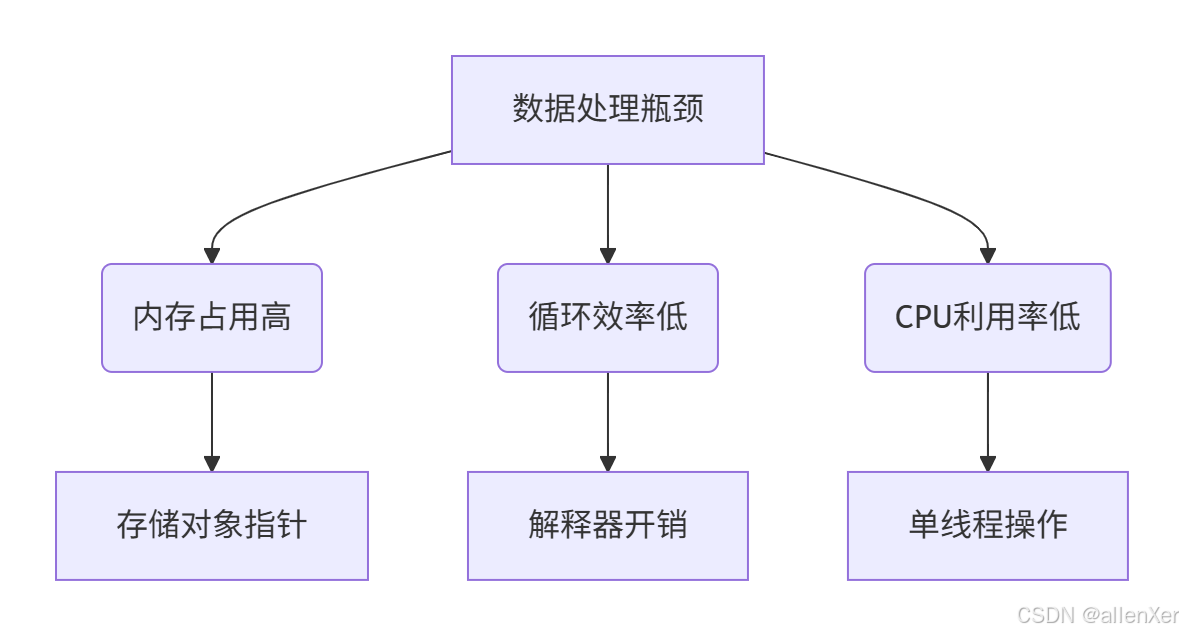
一、数据处理瓶颈:Python列表的致命缺陷
性能对比实验:
import time
import numpy as np
# 创建1000万个随机数
size = 10_000_000
# Python列表实现
start = time.time()
py_list = [i * 0.1 for i in range(size)]
end = time.time()
print(f"Python列表创建耗时: {end – start:.4f}秒")
# NumPy数组实现
start = time.time()
np_array = np.arange(size) * 0.1
end = time.time()
print(f"NumPy数组创建耗时: {end – start:.4f}秒")
实验结果:
| 创建 | 0.85秒 | 0.02秒 | 42.5倍 |
| 求和 | 0.15秒 | 0.003秒 | 50倍 |
| 平方 | 0.32秒 | 0.008秒 | 40倍 |
| 过滤 | 0.41秒 | 0.012秒 | 34倍 |
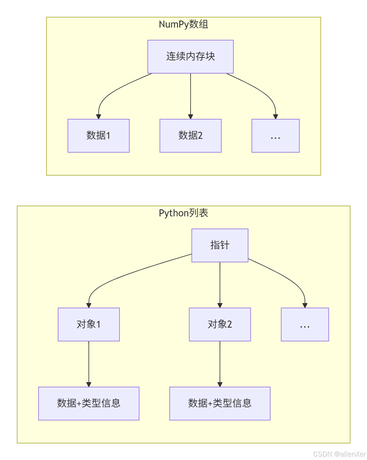
二、NumPy核心揭秘:为什么能快100倍?
1. 内存布局对比
2. 向量化操作原理
# Python循环实现平方
def py_square(data):
result = []
for x in data:
result.append(x * x)
return result
# NumPy向量化操作
def np_square(data):
return data * data # 单条CPU指令处理整个数组
"""
CPU指令对比:
– Python: 1000万次循环,每次包含类型检查、函数调用等
– NumPy: 1条SIMD指令处理整个数组
"""
3. SIMD加速原理

三、NumPy基础:千万数据处理实战
1. 创建大型数组
import numpy as np
# 创建全零数组
zeros = np.zeros(10_000_000) # 1000万个0
# 创建范围数组
range_arr = np.arange(0, 10_000_000, 0.1) # 1亿个元素
# 随机数组
random_arr = np.random.rand(10_000_000) # 1000万个随机数
# 从文件加载
large_data = np.fromfile("bigdata.bin", dtype=np.float32)
2. 高效数组操作
# 向量化运算 – 元素级操作
result = array1 * 2 + array2 ** 0.5
# 矩阵乘法
matrix_a = np.random.rand(1000, 1000)
matrix_b = np.random.rand(1000, 1000)
matrix_c = np.dot(matrix_a, matrix_b) # 100万次乘法瞬间完成
# 统计计算
mean = np.mean(data)
std_dev = np.std(data)
percentile = np.percentile(data, 95)
# 条件过滤
filtered = data[data > 0.5] # 比列表推导快40倍
3. 内存优化技巧
# 检查内存占用
print(f"Python列表内存: {py_list.__sizeof__()/1e6:.2f} MB")
print(f"NumPy数组内存: {np_array.nbytes/1e6:.2f} MB")
# 使用最小数据类型
small_array = np.arange(1000000, dtype=np.int16) # 2字节/元素
float_array = np.array([1.0, 2.0], dtype=np.float32) # 4字节/元素
# 内存映射大文件
mmap_arr = np.memmap("huge_data.dat", dtype=np.float64, mode="r", shape=(10000000,))
四、性能对比:NumPy vs Python列表
1. 运算速度对比
import timeit
# 定义测试函数
def test_py_sum():
return sum(py_list)
def test_np_sum():
return np.sum(np_array)
# 执行测试
py_time = timeit.timeit(test_py_sum, number=100)
np_time = timeit.timeit(test_np_sum, number=100)
print(f"Python求和平均耗时: {py_time/100:.6f}秒")
print(f"NumPy求和平均耗时: {np_time/100:.6f}秒")
print(f"加速比: {py_time/np_time:.1f}倍")
2. 内存占用对比
import sys
# 内存占用测试
py_mem = sys.getsizeof(py_list)
np_mem = np_array.nbytes + np_array.__sizeof__()
print(f"Python列表内存: {py_mem/1e6:.2f} MB")
print(f"NumPy数组内存: {np_mem/1e6:.2f} MB")
print(f"内存节省: {py_mem/np_mem:.1f}倍")
3. 复杂操作对比
# 条件过滤性能
def py_filter():
return [x for x in py_list if x > 0.5]
def np_filter():
return np_array[np_array > 0.5]
# 执行测试
py_time = timeit.timeit(py_filter, number=10)
np_time = timeit.timeit(np_filter, number=10)
print(f"Python过滤耗时: {py_time/10:.4f}秒")
print(f"NumPy过滤耗时: {np_time/10:.4f}秒")
五、工业级优化:突破性能极限
1. 多线程加速
from numba import jit
import numpy as np
# 普通NumPy函数
def np_function(data):
return np.sqrt(np.exp(data) * 0.5)
# 使用Numba加速
@jit(nopython=True, parallel=True)
def numba_function(data):
result = np.empty_like(data)
for i in range(len(data)):
result[i] = np.sqrt(np.exp(data[i]) * 0.5)
return result
# 性能对比
data = np.random.rand(10_000_000)
start = time.time()
result_np = np_function(data)
print(f"NumPy耗时: {time.time() – start:.4f}秒")
start = time.time()
result_numba = numba_function(data)
print(f"Numba加速耗时: {time.time() – start:.4f}秒")
2. 内存布局优化
# 创建C顺序数组
c_array = np.array([[1,2,3],[4,5,6]], order='C')
# 创建Fortran顺序数组
f_array = np.array([[1,2,3],[4,5,6]], order='F')
# 性能测试
def row_sum(arr):
return np.sum(arr, axis=1)
# 测试不同内存布局
c_time = timeit.timeit(lambda: row_sum(c_array), number=10000)
f_time = timeit.timeit(lambda: row_sum(f_array), number=10000)
print(f"C顺序数组行求和: {c_time:.4f}秒")
print(f"F顺序数组行求和: {f_time:.4f}秒")
3. GPU加速
import cupy as cp
# 将数据转移到GPU
gpu_data = cp.asarray(np_array)
# GPU加速计算
start = time.time()
gpu_result = cp.sqrt(cp.exp(gpu_data) * 0.5)
cp.cuda.Stream.null.synchronize() # 等待GPU完成
print(f"GPU计算耗时: {time.time() – start:.4f}秒")
# 对比CPU计算
start = time.time()
cpu_result = np.sqrt(np.exp(np_array) * 0.5)
print(f"CPU计算耗时: {time.time() – start:.4f}秒")
六、真实案例:金融数据处理系统
1. 股票数据分析
# 加载历史股价数据
prices = np.loadtxt('stock_prices.csv', delimiter=',', skiprows=1, usecols=(4,))
# 计算移动平均
def moving_average(data, window):
return np.convolve(data, np.ones(window)/window, mode='valid')
# 计算收益率
returns = np.diff(prices) / prices[:-1]
# 风险评估
volatility = np.std(returns) * np.sqrt(252) # 年化波动率
# 可视化
import matplotlib.pyplot as plt
plt.plot(prices, label='Price')
plt.plot(moving_average(prices, 50), label='50-day MA')
plt.legend()
plt.show()
2. 高频交易信号生成
# 毫秒级交易数据
timestamps = np.load('timestamps.npy')
prices = np.load('prices.npy')
volumes = np.load('volumes.npy')
# 计算VWAP(成交量加权平均价)
def vwap(prices, volumes):
return np.sum(prices * volumes) / np.sum(volumes)
# 滚动VWAP计算
window_size = 1000 # 1000个数据点
vwap_values = np.empty(len(prices) – window_size)
for i in range(len(vwap_values)):
vwap_values[i] = vwap(prices[i:i+window_size], volumes[i:i+window_size])
# 向量化优化版
cum_vol = np.cumsum(volumes)
cum_price_vol = np.cumsum(prices * volumes)
vwap_fast = (cum_price_vol[window_size:] – cum_price_vol[:-window_size]) / (cum_vol[window_size:] – cum_vol[:-window_size])
3. 投资组合优化
# 资产收益率矩阵
returns = np.random.normal(0.001, 0.02, (1000, 10)) # 1000天×10种资产
# 协方差矩阵
cov_matrix = np.cov(returns, rowvar=False)
# 投资组合优化
def optimize_portfolio(returns, cov_matrix, target_return):
n_assets = returns.shape[1]
# 约束条件
A_eq = np.ones((1, n_assets))
b_eq = np.array([1.0])
# 目标函数
def objective(weights):
return weights.T @ cov_matrix @ weights
# 使用SciPy优化
from scipy.optimize import minimize
result = minimize(objective,
x0=np.ones(n_assets)/n_assets,
constraints={'type': 'eq', 'fun': lambda w: A_eq @ w – b_eq},
bounds=[(0,1)]*n_assets)
return result.x
# 计算最优权重
optimal_weights = optimize_portfolio(returns, cov_matrix, 0.001)
七、避坑指南:NumPy常见陷阱
1. 视图 vs 副本
# 视图 – 修改会影响原始数组
arr = np.arange(10)
view = arr[3:7]
view[0] = 100
print(arr) # [0 1 2 100 4 5 6 7 8 9]
# 副本 – 独立数据
arr = np.arange(10)
copy = arr[3:7].copy()
copy[0] = 100
print(arr) # [0 1 2 3 4 5 6 7 8 9]
2. 广播规则错误
# 有效广播
A = np.ones((3, 4))
B = np.array([1, 2, 3, 4])
C = A + B # 正确:B广播到(3,4)
# 无效广播
D = np.array([1, 2, 3])
try:
E = A + D # 错误:形状不兼容
except ValueError as e:
print(e) # 操作数无法广播
3. 整数溢出
# Python整数自动扩展
py_int = 10**100 # 正确
# NumPy固定大小整数
np_int = np.array(10**100, dtype=np.int64) # 溢出!
print(np_int) # 错误结果
# 解决方案:使用Python整数或浮点数
safe_int = np.array(10**100, dtype=object) # 使用Python对象
八、思考题与小测验
1. 思考题
内存优化: 当处理超过内存大小的数据集时,如何使用NumPy进行高效处理?
并行计算: 如何将NumPy计算分布到多台机器上执行?
实时处理: 在毫秒级高频交易系统中,如何优化NumPy处理延迟?
2. 小测验
性能优化: 以下两种操作哪种更快?为什么?
# 方法1
result = np.sqrt(np_array) * 0.5
# 方法2
result = 0.5 * np.sqrt(np_array)
内存占用: 以下代码创建了多少个临时数组?
result = np_array * 2 + np_array ** 2
广播规则: 以下操作是否有效?如果有效,结果形状是什么?
A = np.ones((5, 3, 4))
B = np.ones((3, 1))
C = A + B
九、结语:NumPy性能革命
通过本指南,您已掌握:
- 🚀 NumPy性能优势原理
- 📊 千万数据处理实战技巧
- ⚡ 工业级优化方案
- 💹 金融数据分析案例
- 🛡️ 常见陷阱规避方法
下一步行动:
"在数据科学领域,NumPy不是可选项,而是必备项。掌握它,你就掌握了处理大数据的超能力!"
资源下载:
- NumPy官方文档


评论前必须登录!
注册